Polypropylene (PP/CH2): HNC versus same-potential MD

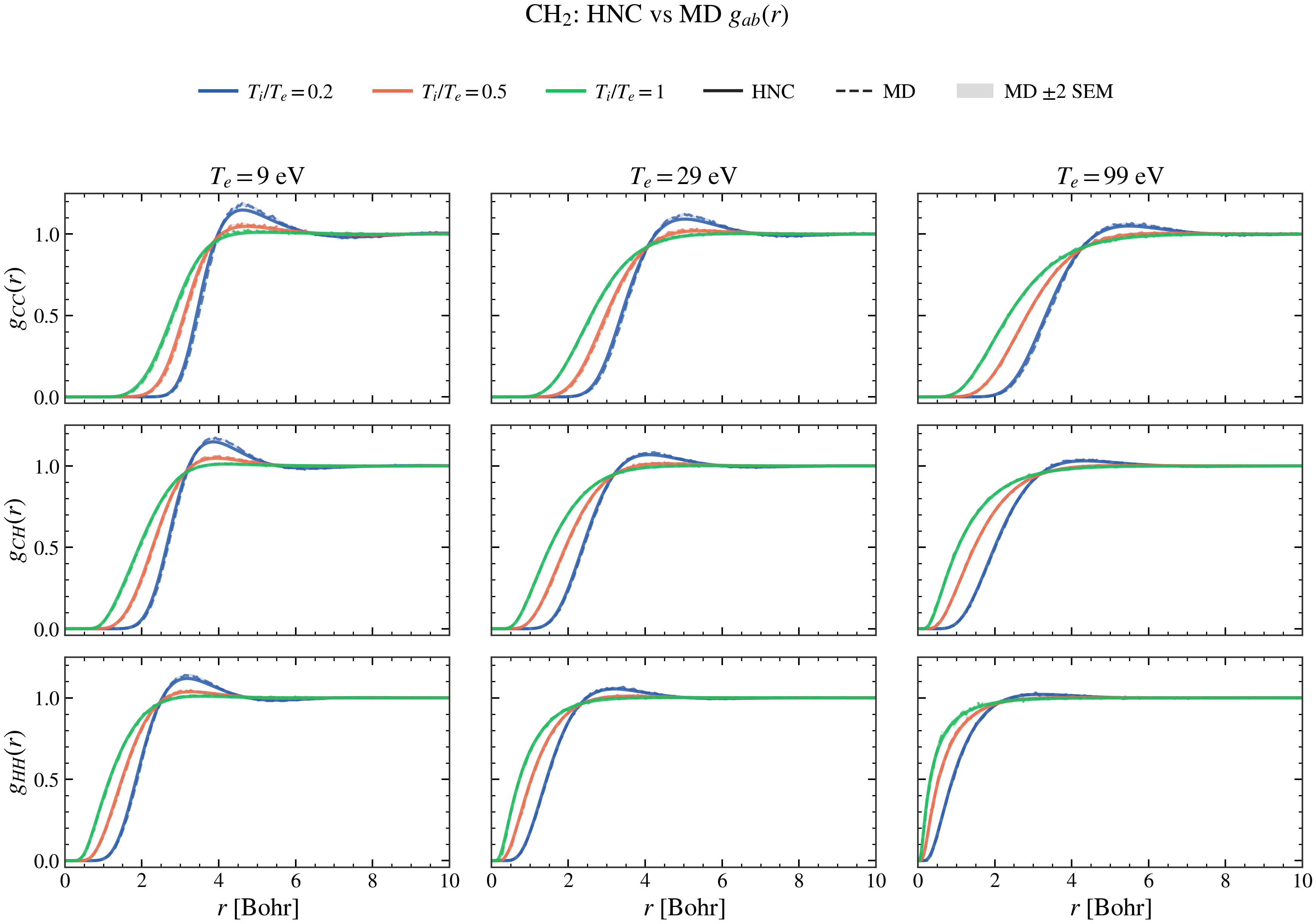
The material is polypropylene (PP), represented in this ion-structure model by its reduced C:H composition, CH2, at \(\rho=0.946\) g cm^-3. The calculation compares Otter multicomponent QOZ/HNC with classical LAMMPS MD [Thompson et al., 2022] at \(T_e=9,29,99\) eV and \(T_i/T_e=0.2,0.5,1.0\). Six of the nine states are explicitly two-temperature states; the three \(T_i/T_e=1\) cases are equilibrium controls. The animation above is an illustrative OVITO rendering of one 3072-ion trajectory and is not used in the numerical comparison.

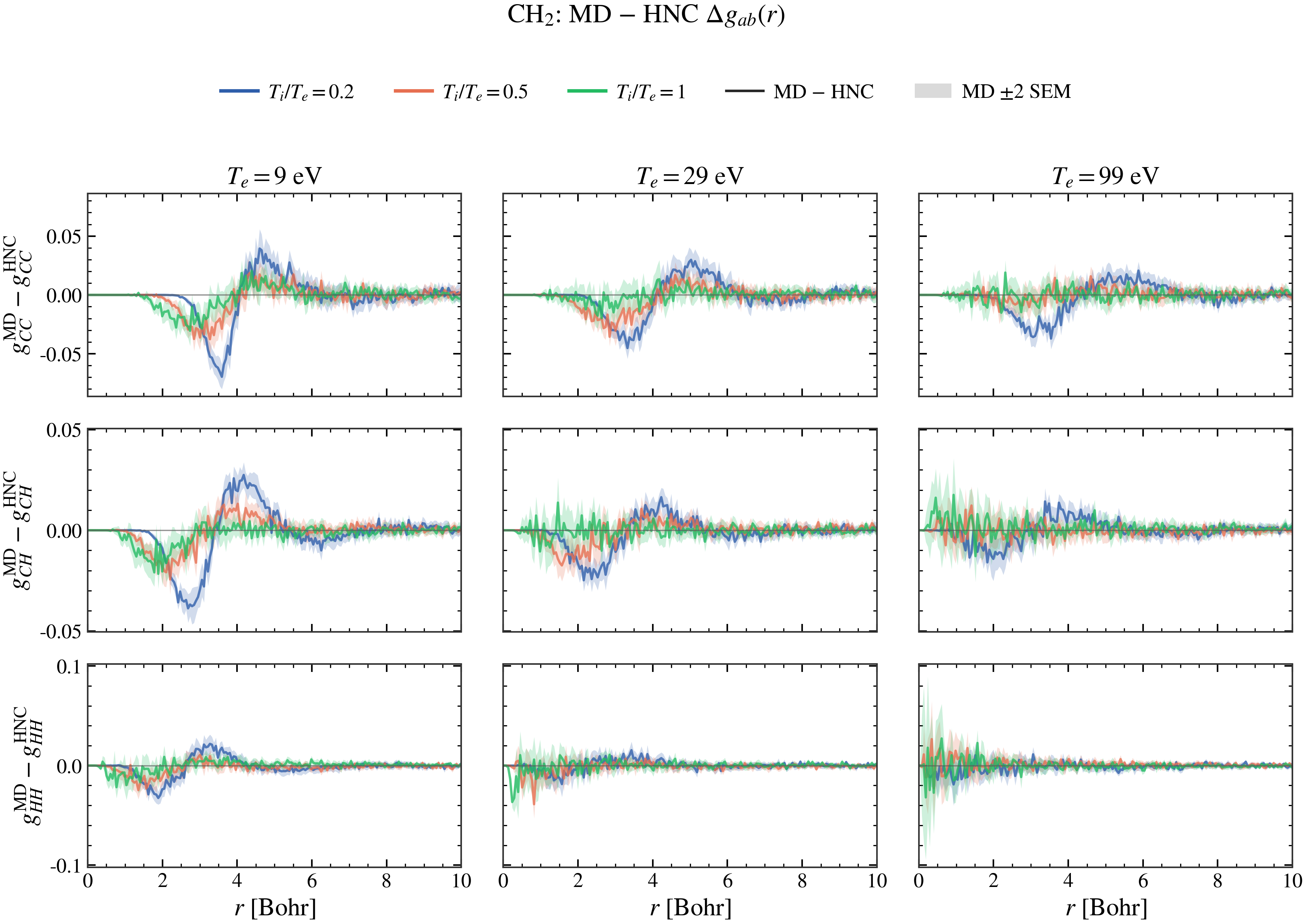
At each electron temperature, one converged IS electronic result is reused for all three ion temperatures. For each state, HNC and MD start from the same QOZ-derived \(V_{ab}^{\mathrm{eff}}(r)\). Ordinary HNC imposes the closure \(B_{ab}(r)=0\) and therefore omits bridge diagrams, whereas MD samples the classical many-ion distribution without imposing that closure. Systematic HNC–MD differences at fixed pair potential therefore primarily test the neglected bridge correlations. Finite cell size, timestep error, and MD sampling uncertainty can also contribute. For the two hottest MD runs only, the analytically known Coulomb core is restored below 0.3 Bohr and blended back to the unchanged QOZ potential by 0.5 Bohr; the resolved first-shell potential is not refitted.

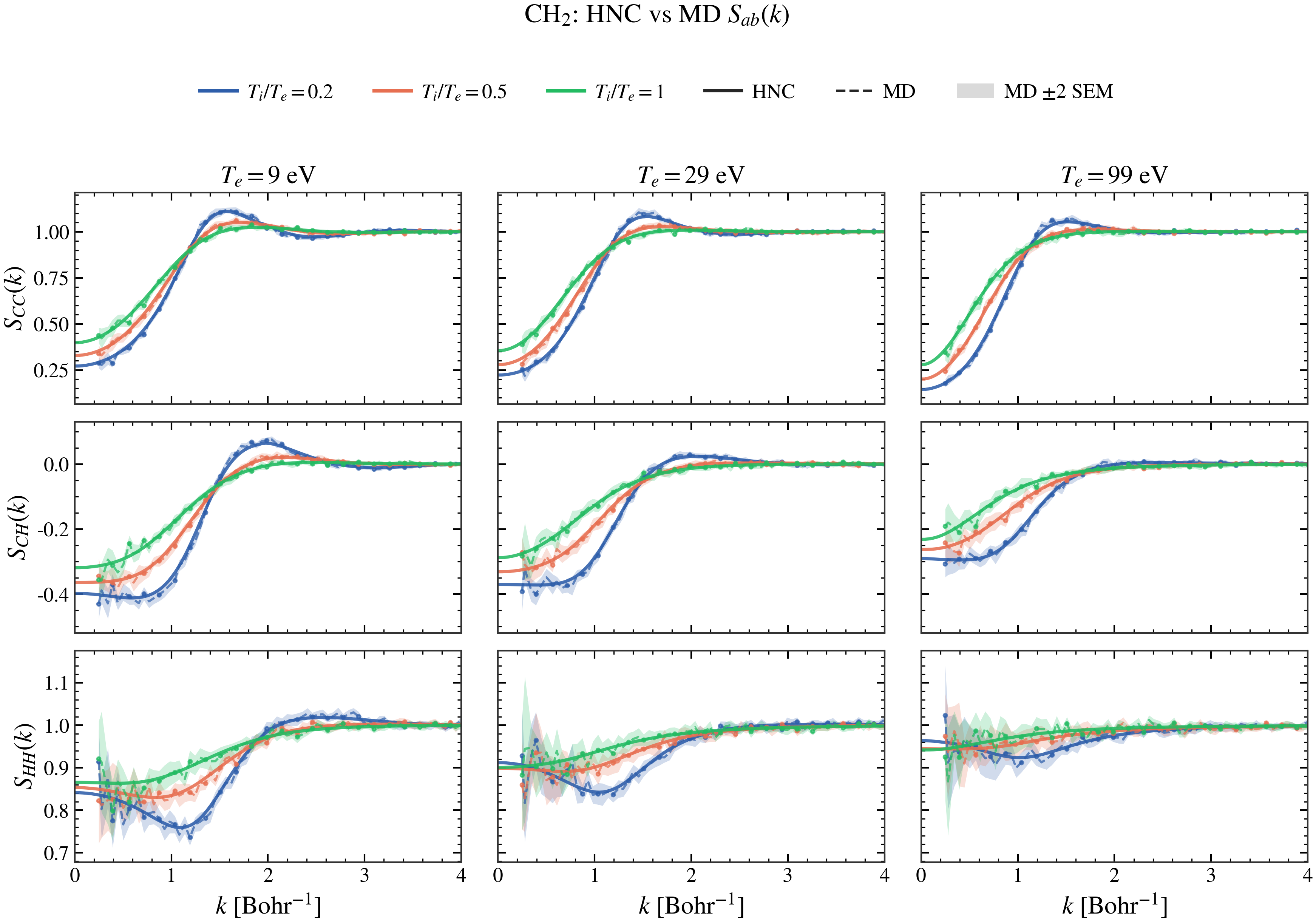
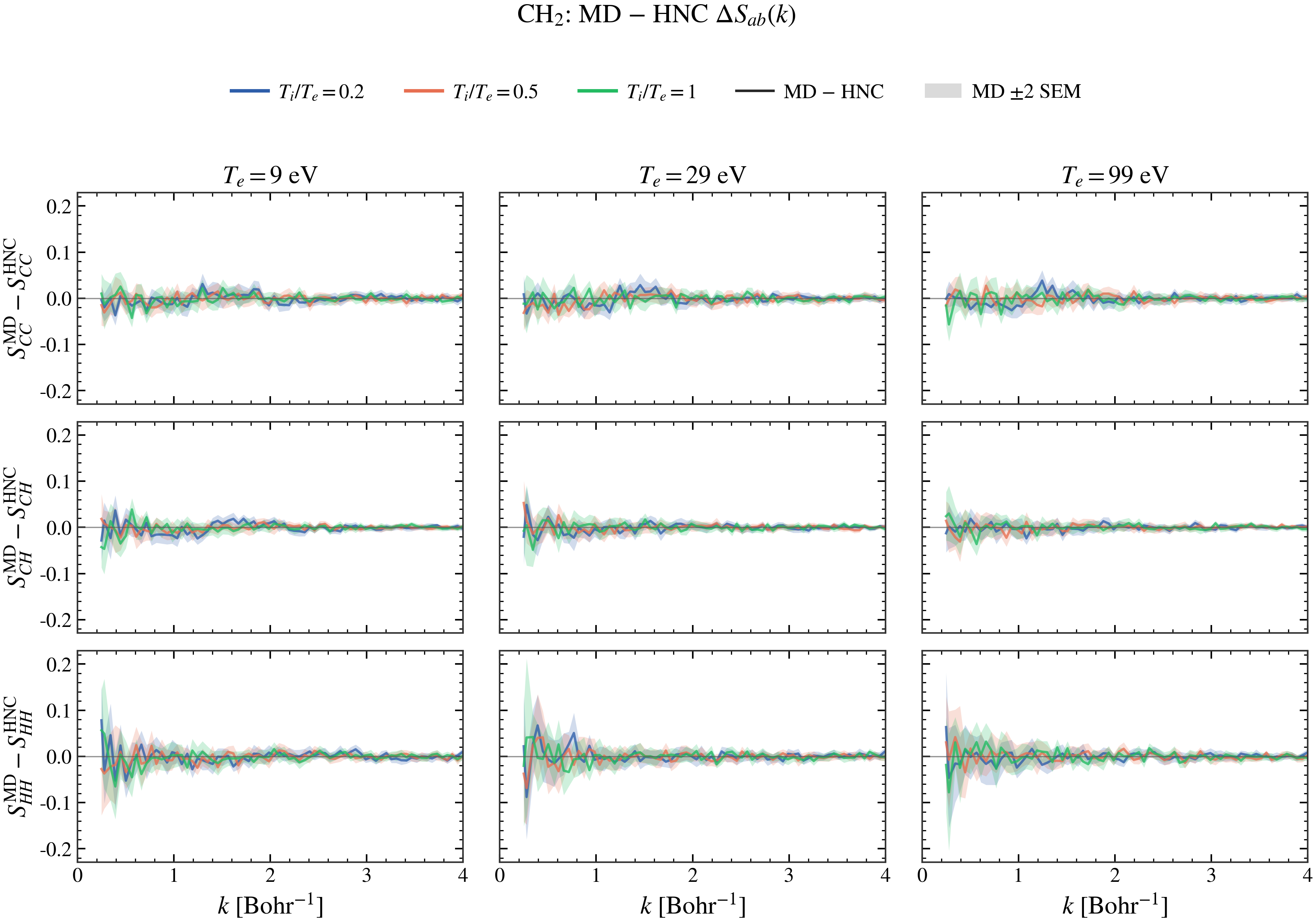
Across the tested window, the pairwise HNC–MD RMSE is \(0.00281\text{--}0.0183\) for \(g_{ab}(r)\) and \(0.00632\text{--}0.0169\) for \(S_{ab}(k)\). HNC takes \(0.38\text{--}1.16\) s per state, while the same-potential MD takes \(8.6\text{--}224\) min. Thus HNC is a good fast approximation for the specific density and temperature range tested here; this is not a universal claim for chemically bonded or more strongly coupled mixtures.

Runtime and MD protocol

Both timings start after the shared \(V_{ab}^{\mathrm{eff}}\) has been prepared: the HNC column is the closure-solver time, while the MD column is the LAMMPS run plus RDF and direct \(S_{ab}(k)\) analysis. Every MD case uses 1024 C and 2048 H ions, NVT equilibration followed by NVE production, and fixed physical durations of \(50\,\omega_p^{-1}\) and \(500\,\omega_p^{-1}\). The thermal timestep guard reduces the two hottest timesteps and increases their step counts accordingly. LAMMPS used 16 MPI ranks with one OpenMP thread per rank (16 concurrent CPU execution threads, reported as a \(2\times2\times4\) processor grid). Direct \(S_{ab}(k)\) post-processing used eight workers. The HNC driver and its BLAS backends were limited to one thread. All states use the same cubic periodic cell with side length 29.322944 Angstrom (55.4123 Bohr) and volume 25,212.895 Angstrom³. The pair-potential cutoff is 14.075013 Angstrom, or \(0.48L\), below the minimum-image limit \(L/2\).

Measured protocol and wall time

States (eV)	\(\Delta t\,\omega_p\)	\(\Delta t\) (ps)	NVT steps	NVE steps	HNC	MD + analysis
First seven: all \(T_e=9,29\); \((T_e,T_i)=(99,19.8)\)	0.005	\(1.3330\times10^{-5}\)	10,000	100,000	0.539–1.164 s	8.57–9.38 min
\((99,49.5)\)	\(4.9945\times10^{-4}\)	\(1.3316\times10^{-6}\)	100,110	1,001,098	0.378 s	179.55 min
\((99,99)\)	\(3.5317\times10^{-4}\)	\(9.4155\times10^{-7}\)	141,577	1,415,766	0.376 s	224.29 min

Summed over the nine independent states, the measured HNC closure time is 6.74 s and the MD-plus-analysis time is 7.76 h. This comparison quantifies the cost of the two ionic-structure treatments after the common electronic potential is available; it does not include that shared electronic/QOZ preparation in either column.

How the MD structure factors are estimated

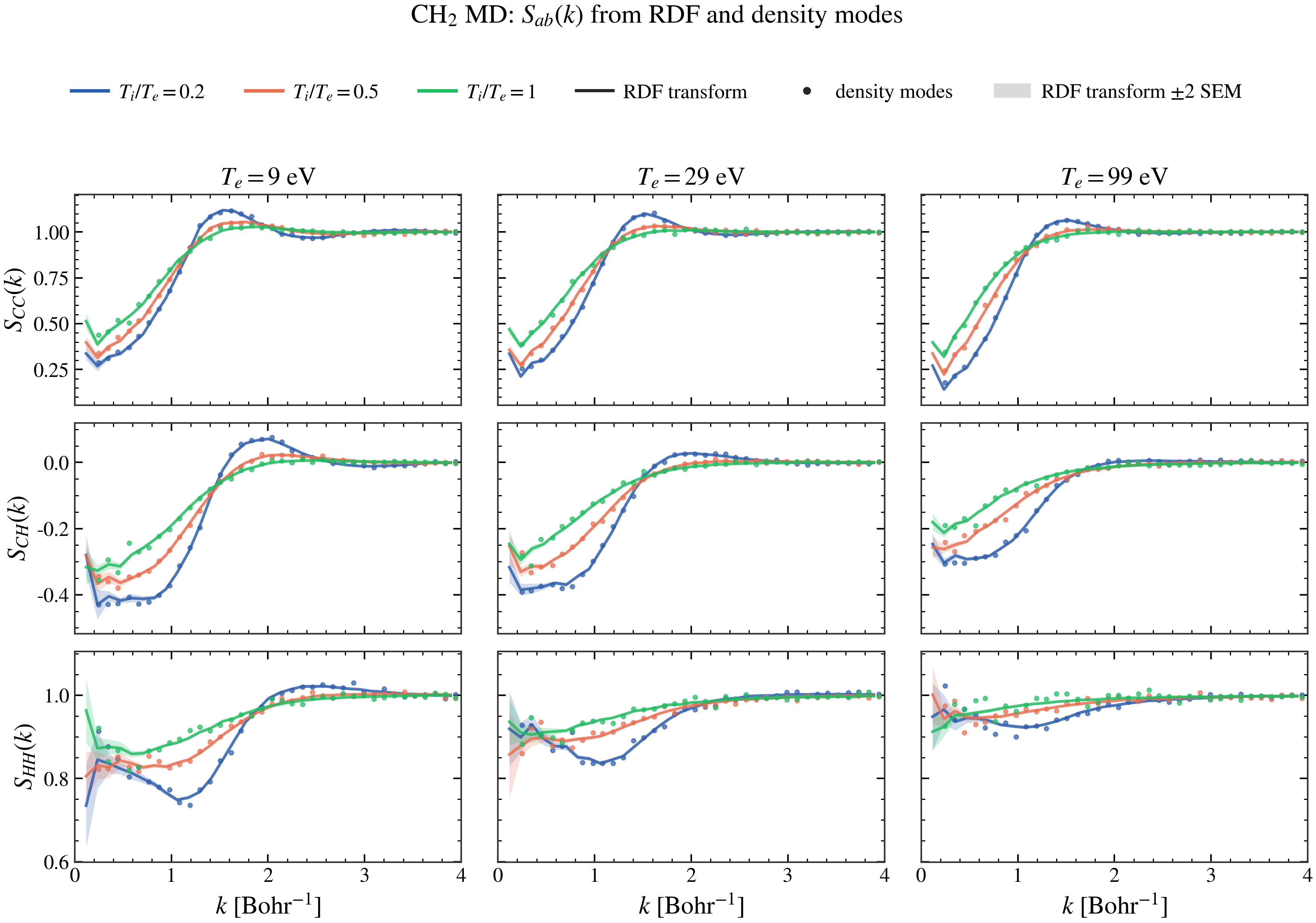
The MD \(S_{ab}(k)\) is evaluated directly from the saved NVE trajectory, not by Fourier transforming the finite-range \(g_{ab}(r)\). For every saved frame \(t\) and nonzero periodic wavevector \(\mathbf{k}=2\pi\mathbf{n}/L\), the species density mode is

\[\rho_a(\mathbf{k},t)=\sum_{j\in a} \exp\!\left[i\mathbf{k}\cdot\mathbf{r}_j(t)\right].\]

The Ashcroft–Langreth partial structure factor is estimated as

\[S_{ab}(k)=\left\langle \frac{\operatorname{Re}\!\left[ \rho_a(\mathbf{k},t)\rho_b^*(\mathbf{k},t)\right]} {\sqrt{N_aN_b}} \right\rangle_{t,\,|\mathbf{k}|\ \mathrm{bin}} .\]

Thus all independent periodic vectors in the same radial \(k\) bin are averaged in each frame, followed by an average over the 21 saved production frames. The shaded band is \(\pm2\,\mathrm{SEM}_{\rm frame}\), where the reported frame SEM is the standard deviation of the per-frame shell averages divided by \(\sqrt{21}\). It does not apply an autocorrelation-time correction, so it should be read as a sampling diagnostic rather than a rigorous confidence interval. Only radial bins containing at least 12 periodic wavevectors are plotted; the omitted smallest-\(k\) bins are the most direction-starved in the finite simulation cell.

As an independent estimator, every one of the 20 LAMMPS RDF blocks is also transformed using Otter’s strict DST-I radial transform,

\[S_{ab}^{g}(k)=\delta_{ab} +\sqrt{n_an_b}\,\mathcal{F}\!\left[g_{ab}(r)-1\right].\]

Each RDF block averages 50 production samples, so this estimator uses 1000 RDF samples rather than the 21 saved coordinate frames used by the direct density modes. LAMMPS reports \(g_{ab}\) at radial-bin centres; the corresponding \(h_{ab}=g_{ab}-1\) is linearly interpolated to the strict \(r_i=i\,\Delta r\) lattice and closed to zero at the first DST point beyond the final RDF centre. Its shaded band is \(\pm2\) SEM across the 20 independently transformed RDF blocks.

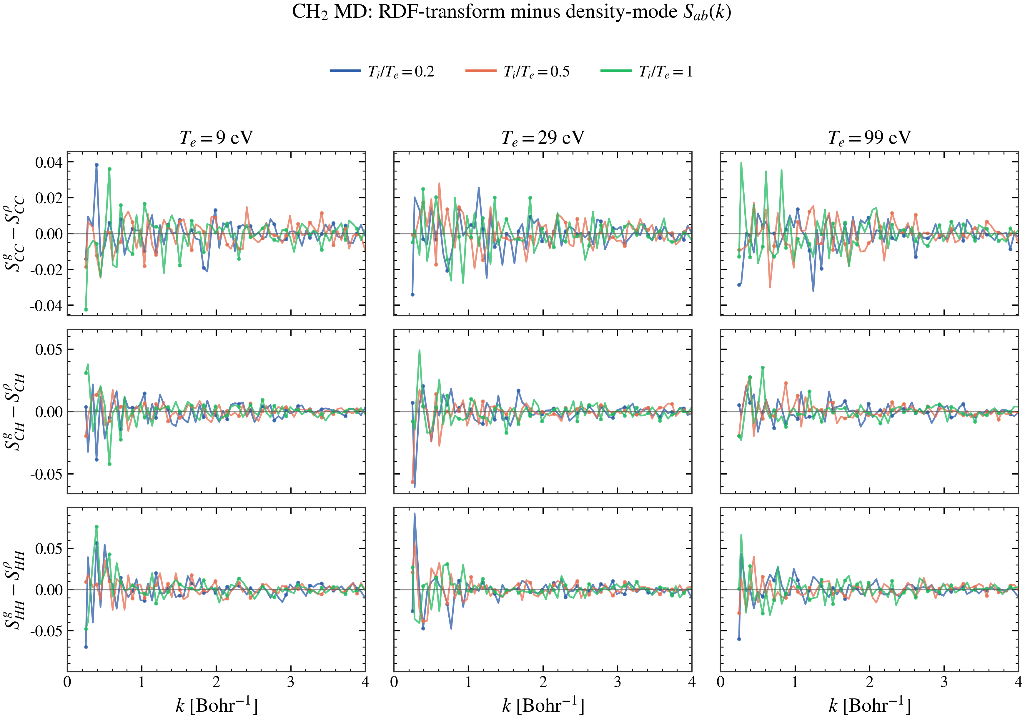
Over the common plotted \(k\) points, the RDF-transform and density-mode estimators have pairwise RMSE \(0.00629\text{--}0.0162\) and an aggregate signed mean difference of \(-6.07\times10^{-5}\). Their main peak shapes therefore agree without a systematic offset. The RDF-transform SEM is about 17–22% of the density-mode SEM because the RDF is sampled much more densely. This smaller statistical band does not include the systematic effect of the finite \(0.48L\) RDF cutoff or the imposed \(h_{ab}=0\) tail; the largest estimator differences remain at the smallest resolved \(k\), especially for \(S_{HH}\).

Data and reproduction

The public, checksummed plotting arrays are stored in benchmarks/baselines/ch2_hnc_md/ch2_hnc_md.npz with their provenance in the adjacent manifest.json. The reusable conversion from Otter \(V_{ab}(r)\) to LAMMPS inputs and the subsequent \(g_{ab}(r)\) and \(S_{ab}(k)\) analysis are implemented in tools/otter_lammps_md.py. Full trajectories and working files are written locally under applications/ch2_xrts_dataset/outputs/ch2_hnc_md_comparison by compare_hnc_md.py; they are too large for the public baseline and are not rerun during documentation builds.

Results

from __future__ import annotations

import hashlib
import json
from pathlib import Path

import matplotlib.pyplot as plt
from matplotlib.lines import Line2D
from matplotlib.patches import Patch
import numpy as np

from otter.plotting import PALETTES, grid_figsize, save_figure, set_style


USE_PRECOMPUTED_DATA = True

BENCHMARK_ID = "ch2_hnc_md"
PAIR_LABELS = ("CC", "CH", "HH")
ALPHA_VALUES = (0.2, 0.5, 1.0)
R_RANGE_BOHR = (0.0, 10.0)
K_RANGE_BOHR_INV = (0.0, 4.0)
MIN_VECTORS_PER_K_BIN = 12
UNCERTAINTY_SIGMA = 2.0
UNCERTAINTY_ALPHA = 0.22


def repository_root() -> Path:
    """Locate the checkout in direct and Sphinx-Gallery execution modes."""
    candidates = [Path.cwd().resolve(), *Path.cwd().resolve().parents]
    source = Path(str(globals().get("__file__", Path.cwd()))).resolve()
    candidates.extend([source.parent, *source.parents])
    for candidate in candidates:
        if (candidate / "pyproject.toml").is_file() and (
            candidate / "benchmarks" / "baselines" / BENCHMARK_ID
        ).is_dir():
            return candidate
    raise FileNotFoundError("Cannot locate the Otter checkout.")


def sha256_file(path: Path) -> str:
    """Return a streaming SHA-256 digest."""
    digest = hashlib.sha256()
    with path.open("rb") as stream:
        for block in iter(lambda: stream.read(1024 * 1024), b""):
            digest.update(block)
    return digest.hexdigest()


ROOT = repository_root()
BASELINE_DIR = ROOT / "benchmarks" / "baselines" / BENCHMARK_ID
OUTPUT_DIR = ROOT / "benchmarks" / "outputs" / BENCHMARK_ID
FIGURE_DIR = OUTPUT_DIR / "figures"


def load_baseline() -> dict[str, np.ndarray]:
    """Verify the accepted numerical archive and bundled media checksums."""
    if not USE_PRECOMPUTED_DATA:
        raise RuntimeError(
            "Run applications/ch2_xrts_dataset/compare_hnc_md.py to create "
            "fresh long-running candidates; this gallery never overwrites "
            "the accepted baseline."
        )
    manifest = json.loads(
        (BASELINE_DIR / "manifest.json").read_text(encoding="utf-8")
    )
    if manifest.get("benchmark_id") != BENCHMARK_ID:
        raise ValueError("Unexpected CH2 HNC--MD benchmark manifest.")
    record = manifest["baseline"]
    path = BASELINE_DIR / str(record["path"])
    if sha256_file(path) != str(record["sha256"]):
        raise RuntimeError(f"Checksum mismatch for {path}.")
    for media in manifest["media"]:
        media_path = ROOT / str(media["path"])
        if sha256_file(media_path) != str(media["sha256"]):
            raise RuntimeError(f"Checksum mismatch for {media_path}.")
    with np.load(path, allow_pickle=False) as archive:
        payload = {key: np.asarray(archive[key]) for key in archive.files}
    if str(payload["schema_version"].item()) != "otter_ch2_hnc_md_v2":
        raise ValueError("Obsolete CH2 HNC--MD baseline schema.")
    if payload["te_ev"].shape != (9,) or np.count_nonzero(
        ~np.isclose(payload["alpha"], 1.0)
    ) != 6:
        raise ValueError("Expected nine states, including six non-equilibrium states.")
    return payload


data = load_baseline()
print("Loaded nine checksummed HNC--MD states (six two-temperature states).")


def alpha_handles() -> list[object]:
    """Return shared temperature-ratio legend handles."""
    return [
        Line2D(
            [], [], color=ALPHA_COLORS[alpha], lw=2.2,
            label=rf"$T_i/T_e={alpha:g}$",
        )
        for alpha in ALPHA_VALUES
    ]


def comparison_handles() -> list[object]:
    """Return the common method and uncertainty legend."""
    return alpha_handles() + [
        Line2D([], [], color="0.15", lw=2.0, ls="-", label="HNC"),
        Line2D([], [], color="0.15", lw=1.6, ls="--", label="MD"),
        Patch(
            facecolor="0.35", alpha=UNCERTAINTY_ALPHA, edgecolor="none",
            label=r"MD $\pm2$ SEM",
        ),
    ]


def estimator_handles() -> list[object]:
    """Return the RDF-transform and direct-density estimator legend."""
    return alpha_handles() + [
        Line2D([], [], color="0.15", lw=2.0, label="RDF transform"),
        Line2D(
            [], [], color="0.15", lw=0.0, marker="o", ms=4.0,
            label="density modes",
        ),
        Patch(
            facecolor="0.35", alpha=UNCERTAINTY_ALPHA, edgecolor="none",
            label=r"RDF transform $\pm2$ SEM",
        ),
    ]


def finish_grid(fig: object, title: str, handles: list[object]) -> None:
    """Apply the shared compact title and top legend layout."""
    fig.suptitle(title, y=0.99)
    fig.legend(
        handles=handles, loc="upper center", bbox_to_anchor=(0.5, 0.925),
        ncol=len(handles), frameon=False,
    )
    fig.tight_layout(rect=(0.0, 0.0, 1.0, 0.90), h_pad=0.8, w_pad=1.2)


TE_VALUES = tuple(float(value) for value in np.unique(data["te_ev"]))
ALPHA_COLORS = dict(zip(ALPHA_VALUES, PALETTES["bing"][1:4], strict=True))
set_style("thesis", palette="bing")

Loaded nine checksummed HNC--MD states (six two-temperature states).

Pair distributions

fig_g, axes = plt.subplots(
    3, 3, figsize=grid_figsize(3, 3), sharex=True, sharey=True
)
for column, te_ev in enumerate(TE_VALUES):
    axes[0, column].set_title(rf"$T_e={te_ev:g}$ eV")
    for state in np.flatnonzero(np.isclose(data["te_ev"], te_ev)):
        alpha = float(data["alpha"][state])
        color = ALPHA_COLORS[alpha]
        for pair, label in enumerate(PAIR_LABELS):
            axes[pair, column].plot(
                data["hnc_r_bohr"][state], data["hnc_gij_r"][state, pair],
                color=color, lw=2.0, alpha=0.88,
            )
            g_md = data["md_gij_r"][state, pair]
            sem = data["md_gij_sem"][state, pair]
            axes[pair, column].plot(
                data["md_r_bohr"], g_md, color=color, lw=1.6,
                ls="--", alpha=0.76,
            )
            axes[pair, column].fill_between(
                data["md_r_bohr"],
                g_md - UNCERTAINTY_SIGMA * sem,
                g_md + UNCERTAINTY_SIGMA * sem,
                color=color, alpha=UNCERTAINTY_ALPHA, linewidth=0.0,
            )
for row, label in enumerate(PAIR_LABELS):
    axes[row, 0].set_ylabel(rf"$g_{{{label}}}(r)$")
for axis in axes[-1]:
    axis.set_xlabel(r"$r$ [Bohr]")
for axis in axes.flat:
    axis.set(xlim=R_RANGE_BOHR, ylim=(-0.04, 1.25))
finish_grid(fig_g, r"CH$_2$: HNC vs MD $g_{ab}(r)$", comparison_handles())
_ = save_figure(fig_g, FIGURE_DIR / "ch2_hnc_md_gab", close=True)

Pair-distribution residuals

fig_gd, axes = plt.subplots(
    3, 3, figsize=grid_figsize(3, 3), sharex=True, sharey="row"
)
g_residual_extent: list[list[np.ndarray]] = [[], [], []]
g_visible = data["md_r_bohr"] <= R_RANGE_BOHR[1]
for column, te_ev in enumerate(TE_VALUES):
    axes[0, column].set_title(rf"$T_e={te_ev:g}$ eV")
    for state in np.flatnonzero(np.isclose(data["te_ev"], te_ev)):
        alpha = float(data["alpha"][state])
        color = ALPHA_COLORS[alpha]
        for pair, label in enumerate(PAIR_LABELS):
            hnc = np.interp(
                data["md_r_bohr"], data["hnc_r_bohr"][state],
                data["hnc_gij_r"][state, pair],
            )
            delta = data["md_gij_r"][state, pair] - hnc
            sem = data["md_gij_sem"][state, pair]
            g_residual_extent[pair].append(
                np.abs(delta[g_visible]) + UNCERTAINTY_SIGMA * sem[g_visible]
            )
            axes[pair, column].plot(
                data["md_r_bohr"], delta, color=color, lw=1.5, alpha=0.78,
            )
            axes[pair, column].fill_between(
                data["md_r_bohr"],
                delta - UNCERTAINTY_SIGMA * sem,
                delta + UNCERTAINTY_SIGMA * sem,
                color=color, alpha=UNCERTAINTY_ALPHA, linewidth=0.0,
            )
for row, label in enumerate(PAIR_LABELS):
    axes[row, 0].set_ylabel(
        r"$g_{%s}^{\mathrm{MD}}-g_{%s}^{\mathrm{HNC}}$" % (label, label)
    )
    row_limit = 1.08 * max(
        float(np.max(values)) for values in g_residual_extent[row]
    )
    for axis in axes[row]:
        axis.set_ylim(-row_limit, row_limit)
for axis in axes[-1]:
    axis.set_xlabel(r"$r$ [Bohr]")
for axis in axes.flat:
    axis.axhline(0.0, color="0.35", lw=0.8, alpha=0.65)
    axis.set_xlim(*R_RANGE_BOHR)
finish_grid(
    fig_gd,
    r"CH$_2$: MD $-$ HNC $\Delta g_{ab}(r)$",
    alpha_handles() + [
        Line2D([], [], color="0.15", lw=1.6, label="MD $-$ HNC"),
        Patch(
            facecolor="0.35", alpha=UNCERTAINTY_ALPHA, edgecolor="none",
            label=r"MD $\pm2$ SEM",
        ),
    ],
)
_ = save_figure(
    fig_gd, FIGURE_DIR / "ch2_hnc_md_gab_residual", close=True
)

Partial structure factors

fig_s, axes = plt.subplots(
    3, 3, figsize=grid_figsize(3, 3), sharex=True, sharey="row"
)
reliable = data["md_vectors_per_k_bin"] >= MIN_VECTORS_PER_K_BIN
for column, te_ev in enumerate(TE_VALUES):
    axes[0, column].set_title(rf"$T_e={te_ev:g}$ eV")
    for state in np.flatnonzero(np.isclose(data["te_ev"], te_ev)):
        alpha = float(data["alpha"][state])
        color = ALPHA_COLORS[alpha]
        for pair, label in enumerate(PAIR_LABELS):
            axes[pair, column].plot(
                data["hnc_k_bohr_inv"][state],
                data["hnc_sij_k"][state, pair],
                color=color, lw=2.0, alpha=0.88,
            )
            s_md = data["md_sij_k"][state, pair, reliable]
            sem = data["md_sij_sem"][state, pair, reliable]
            k_md = data["md_k_bohr_inv"][reliable]
            axes[pair, column].plot(
                k_md, s_md, color=color, lw=1.4, ls="--", marker="o",
                ms=2.3, markevery=3, alpha=0.72,
            )
            axes[pair, column].fill_between(
                k_md,
                s_md - UNCERTAINTY_SIGMA * sem,
                s_md + UNCERTAINTY_SIGMA * sem,
                color=color, alpha=UNCERTAINTY_ALPHA, linewidth=0.0,
            )
for row, label in enumerate(PAIR_LABELS):
    axes[row, 0].set_ylabel(rf"$S_{{{label}}}(k)$")
for axis in axes[-1]:
    axis.set_xlabel(r"$k$ [Bohr$^{-1}$]")
for axis in axes.flat:
    axis.set_xlim(*K_RANGE_BOHR_INV)
    axis.margins(y=0.08)
finish_grid(fig_s, r"CH$_2$: HNC vs MD $S_{ab}(k)$", comparison_handles())
_ = save_figure(fig_s, FIGURE_DIR / "ch2_hnc_md_sab", close=True)

Structure-factor residuals

fig_d, axes = plt.subplots(
    3, 3, figsize=grid_figsize(3, 3), sharex=True, sharey=True
)
residual_extent: list[np.ndarray] = []
visible = reliable & (data["md_k_bohr_inv"] <= K_RANGE_BOHR_INV[1])
for column, te_ev in enumerate(TE_VALUES):
    axes[0, column].set_title(rf"$T_e={te_ev:g}$ eV")
    for state in np.flatnonzero(np.isclose(data["te_ev"], te_ev)):
        alpha = float(data["alpha"][state])
        color = ALPHA_COLORS[alpha]
        for pair, label in enumerate(PAIR_LABELS):
            hnc = np.interp(
                data["md_k_bohr_inv"], data["hnc_k_bohr_inv"][state],
                data["hnc_sij_k"][state, pair],
            )
            delta = data["md_sij_k"][state, pair] - hnc
            sem = data["md_sij_sem"][state, pair]
            residual_extent.append(
                np.abs(delta[visible]) + UNCERTAINTY_SIGMA * sem[visible]
            )
            axes[pair, column].plot(
                data["md_k_bohr_inv"][reliable], delta[reliable],
                color=color, lw=1.5, alpha=0.78,
            )
            axes[pair, column].fill_between(
                data["md_k_bohr_inv"][reliable],
                delta[reliable] - UNCERTAINTY_SIGMA * sem[reliable],
                delta[reliable] + UNCERTAINTY_SIGMA * sem[reliable],
                color=color, alpha=UNCERTAINTY_ALPHA, linewidth=0.0,
            )
limit = 1.08 * max(float(np.max(values)) for values in residual_extent)
for row, label in enumerate(PAIR_LABELS):
    axes[row, 0].set_ylabel(
        r"$S_{%s}^{\mathrm{MD}}-S_{%s}^{\mathrm{HNC}}$" % (label, label)
    )
for axis in axes[-1]:
    axis.set_xlabel(r"$k$ [Bohr$^{-1}$]")
for axis in axes.flat:
    axis.axhline(0.0, color="0.35", lw=0.8, alpha=0.65)
    axis.set(xlim=K_RANGE_BOHR_INV, ylim=(-limit, limit))
finish_grid(
    fig_d,
    r"CH$_2$: MD $-$ HNC $\Delta S_{ab}(k)$",
    alpha_handles() + [
        Line2D([], [], color="0.15", lw=1.6, label="MD $-$ HNC"),
        Patch(
            facecolor="0.35", alpha=UNCERTAINTY_ALPHA, edgecolor="none",
            label=r"MD $\pm2$ SEM",
        ),
    ],
)
_ = save_figure(fig_d, FIGURE_DIR / "ch2_hnc_md_sab_residual", close=True)

MD structure-factor estimators

fig_e, axes = plt.subplots(
    3, 3, figsize=grid_figsize(3, 3), sharex=True, sharey="row"
)
rdf_visible = data["md_rdf_k_bohr_inv"] <= K_RANGE_BOHR_INV[1]
for column, te_ev in enumerate(TE_VALUES):
    axes[0, column].set_title(rf"$T_e={te_ev:g}$ eV")
    for state in np.flatnonzero(np.isclose(data["te_ev"], te_ev)):
        alpha = float(data["alpha"][state])
        color = ALPHA_COLORS[alpha]
        for pair, label in enumerate(PAIR_LABELS):
            s_rdf = data["md_sij_from_rdf"][state, pair]
            sem_rdf = data["md_sij_from_rdf_sem"][state, pair]
            axes[pair, column].plot(
                data["md_rdf_k_bohr_inv"][rdf_visible],
                s_rdf[rdf_visible], color=color, lw=1.8, alpha=0.82,
            )
            axes[pair, column].fill_between(
                data["md_rdf_k_bohr_inv"][rdf_visible],
                s_rdf[rdf_visible] - UNCERTAINTY_SIGMA * sem_rdf[rdf_visible],
                s_rdf[rdf_visible] + UNCERTAINTY_SIGMA * sem_rdf[rdf_visible],
                color=color, alpha=UNCERTAINTY_ALPHA, linewidth=0.0,
            )
            axes[pair, column].plot(
                data["md_k_bohr_inv"][reliable],
                data["md_sij_k"][state, pair, reliable],
                color=color, lw=0.0, marker="o", ms=2.5,
                markevery=2, alpha=0.66,
            )
for row, label in enumerate(PAIR_LABELS):
    axes[row, 0].set_ylabel(rf"$S_{{{label}}}(k)$")
for axis in axes[-1]:
    axis.set_xlabel(r"$k$ [Bohr$^{-1}$]")
for axis in axes.flat:
    axis.set_xlim(*K_RANGE_BOHR_INV)
    axis.margins(y=0.08)
finish_grid(
    fig_e,
    r"CH$_2$ MD: $S_{ab}(k)$ from RDF and density modes",
    estimator_handles(),
)
_ = save_figure(
    fig_e, FIGURE_DIR / "ch2_md_sab_rdf_vs_density", close=True
)

Difference between the MD estimators

fig_ed, axes = plt.subplots(
    3, 3, figsize=grid_figsize(3, 3), sharex=True, sharey="row"
)
estimator_extent: list[list[np.ndarray]] = [[], [], []]
estimator_visible = (
    reliable
    & (data["md_k_bohr_inv"] >= data["md_rdf_k_bohr_inv"][0])
    & (data["md_k_bohr_inv"] <= K_RANGE_BOHR_INV[1])
)
for column, te_ev in enumerate(TE_VALUES):
    axes[0, column].set_title(rf"$T_e={te_ev:g}$ eV")
    for state in np.flatnonzero(np.isclose(data["te_ev"], te_ev)):
        alpha = float(data["alpha"][state])
        color = ALPHA_COLORS[alpha]
        k_compare = data["md_k_bohr_inv"][estimator_visible]
        for pair, label in enumerate(PAIR_LABELS):
            s_rdf = np.interp(
                k_compare,
                data["md_rdf_k_bohr_inv"],
                data["md_sij_from_rdf"][state, pair],
            )
            difference = (
                s_rdf - data["md_sij_k"][state, pair, estimator_visible]
            )
            estimator_extent[pair].append(np.abs(difference))
            axes[pair, column].plot(
                k_compare, difference, color=color, lw=1.4, marker="o",
                ms=2.2, markevery=3, alpha=0.76,
            )
for row, label in enumerate(PAIR_LABELS):
    axes[row, 0].set_ylabel(
        r"$S_{%s}^{g}-S_{%s}^{\rho}$" % (label, label)
    )
    row_limit = 1.08 * max(
        float(np.max(values)) for values in estimator_extent[row]
    )
    for axis in axes[row]:
        axis.set_ylim(-row_limit, row_limit)
for axis in axes[-1]:
    axis.set_xlabel(r"$k$ [Bohr$^{-1}$]")
for axis in axes.flat:
    axis.axhline(0.0, color="0.35", lw=0.8, alpha=0.65)
    axis.set_xlim(*K_RANGE_BOHR_INV)
finish_grid(
    fig_ed,
    r"CH$_2$ MD: RDF-transform minus density-mode $S_{ab}(k)$",
    alpha_handles(),
)
_ = save_figure(
    fig_ed, FIGURE_DIR / "ch2_md_sab_rdf_minus_density", close=True
)


print(
    "HNC seconds: "
    f"{np.min(data['hnc_elapsed_s']):.3f}--{np.max(data['hnc_elapsed_s']):.3f}; "
    "MD minutes: "
    f"{np.min(data['md_elapsed_s']) / 60.0:.2f}--"
    f"{np.max(data['md_elapsed_s']) / 60.0:.2f}."
)
print(
    "Pairwise RMSE ranges: "
    f"g={np.min(data['g_rmse']):.5f}--{np.max(data['g_rmse']):.5f}; "
    f"S={np.min(data['s_rmse']):.5f}--{np.max(data['s_rmse']):.5f}."
)
print(
    "RDF-transform versus density-mode S(k): "
    f"RMSE={np.min(data['md_sij_estimator_rmse']):.5f}--"
    f"{np.max(data['md_sij_estimator_rmse']):.5f}; "
    "aggregate signed mean="
    f"{np.mean(data['md_sij_estimator_signed_mean']):+.3e}; "
    f"max abs={np.max(data['md_sij_estimator_max_abs']):.5f}."
)

if "agg" not in plt.get_backend().lower():
    plt.show()

HNC seconds: 0.376--1.164; MD minutes: 8.57--224.29.
Pairwise RMSE ranges: g=0.00281--0.01826; S=0.00632--0.01694.
RDF-transform versus density-mode S(k): RMSE=0.00629--0.01616; aggregate signed mean=-6.075e-05; max abs=0.09243.