Note
Go to the end to download the full example code.
Carbon: local-field-correction sensitivity
This complete example keeps the carbon KS average atom and screening cloud
fixed, then changes only the static electron local-field correction (LFC) in
the response, effective ion potential, and HNC calculation. The state is
rho=5 g/cc at T=2 and 100 eV.
The pseudoatom/QOZ construction follows Starrett and Saumon [2014]. The
models are RPA, Hubbard [Hubbard, 1958], Utsumi–Ichimaru
[Utsumi and Ichimaru, 1982], Chabrier-1990 [Chabrier, 1990], and the
Gregori interpolation [Geldart and Vosko, 1966, Gregori et al., 2007]. Otter’s
Gregori/Geldart–Vosko implementation is an attributed NumPy port from
JaXRTS [Lütgert et al., 2026]; the exact revision and BSD-3-Clause notice
are recorded in THIRD_PARTY_NOTICES.md.
Set RECOMPUTE_WITH_OTTER=True below to run the shared electronic state and
all five ion-structure branches directly through Otter’s public API. The
default verifies and loads reviewed Otter results so documentation builds
remain quick.
Further numerical definitions and interpretation are given in the LFC model-study notes.
from __future__ import annotations

from concurrent.futures import ProcessPoolExecutor, as_completed
import hashlib
import json
import os
from pathlib import Path
import time
from typing import Any

import matplotlib.pyplot as plt
import numpy as np

from otter import (
    PlasmaWorkflowConfig,
    continue_plasma_workflow_from_electronic_result,
    solve_plasma_workflow,
)
from otter.ionic import decompose_effective_pair_potential_k
from otter.plotting import grid_figsize, save_figure, style_context


# =============================================================================
# User input
# =============================================================================
RECOMPUTE_WITH_OTTER = False
if os.environ.get("OTTER_RECOMPUTE_CARBON_LFC", "0") == "1":
    RECOMPUTE_WITH_OTTER = True

# Use the ionic comparison as the gallery-card preview.
sphinx_gallery_thumbnail_number = 3

RHO_G_CC = 5.0
TEMPERATURES_EV = (2.0, 100.0)
LFC_MODELS = (
    "none",
    "hubbard",
    "utsumiichimaru",
    "chabrier1990",
    "gregori2007",
)
REFERENCE_LFC = "chabrier1990"

MAX_STATE_WORKERS = 2
CONTINUUM_WORKERS_PER_STATE = 6
QOZ_N_POINTS = 8192
HNC_TOL = 1.0e-5
HNC_CLOSURE_TOL = 1.0e-4
R_RETAIN_MAX_BOHR = 20.0
K_RETAIN_MAX_BOHR_INV = 20.0
LOW_K_PLOT_MAX_BOHR_INV = 1.2
# =============================================================================


MODEL_LABELS = {
    "none": "RPA",
    "hubbard": "Hubbard",
    "utsumiichimaru": "Utsumi–Ichimaru",
    "chabrier1990": "Chabrier-1990",
    "gregori2007": "Gregori interpolation",
}


def repository_root() -> Path:
    """Locate the checkout when run directly or through Sphinx-Gallery."""
    candidates = [Path.cwd().resolve(), *Path.cwd().resolve().parents]
    source_file = globals().get("__file__")
    if source_file is not None:
        source = Path(str(source_file)).resolve()
        candidates.extend([source.parent, *source.parents])
    for candidate in candidates:
        manifest = (
            candidate
            / "benchmarks"
            / "baselines"
            / "carbon_lfc_sensitivity"
            / "manifest.json"
        )
        if manifest.is_file():
            return candidate
    raise FileNotFoundError("Cannot locate the Otter checkout.")


ROOT = repository_root()
BASELINE_DIR = ROOT / "benchmarks" / "baselines" / "carbon_lfc_sensitivity"
OUTPUT_DIR = ROOT / "benchmarks" / "outputs" / "carbon_lfc_sensitivity"
CANDIDATE_DIR = OUTPUT_DIR / "gallery_recomputed"
FIGURE_DIR = OUTPUT_DIR / "figures"


def sha256_file(path: Path) -> str:
    """Return a streaming SHA-256 digest."""
    digest = hashlib.sha256()
    with path.open("rb") as stream:
        for block in iter(lambda: stream.read(1024 * 1024), b""):
            digest.update(block)
    return digest.hexdigest()


def load_npz(path: Path) -> dict[str, np.ndarray]:
    """Load a portable archive without enabling object deserialization."""
    with np.load(path, allow_pickle=False) as archive:
        state = {key: np.asarray(archive[key]) for key in archive.files}
    if any(value.dtype.hasobject for value in state.values()):
        raise TypeError(f"Object arrays are forbidden in {path}.")
    return state


def load_reviewed_states() -> list[dict[str, np.ndarray]]:
    """Verify and load the accepted current-Otter calculations."""
    manifest_path = BASELINE_DIR / "manifest.json"
    manifest = json.loads(manifest_path.read_text(encoding="utf-8"))
    if manifest.get("benchmark_id") != "carbon_lfc_sensitivity":
        raise ValueError("Unexpected carbon LFC manifest.")
    states: list[dict[str, np.ndarray]] = []
    for record in manifest["states"]:
        path = BASELINE_DIR / str(record["data_file"])
        if sha256_file(path) != str(record["data_sha256"]):
            raise RuntimeError(f"Checksum mismatch for {path}.")
        state = load_npz(path)
        if tuple(str(value) for value in state["model_labels"]) != LFC_MODELS:
            raise ValueError(f"Unexpected LFC model order in {path}.")
        states.append(state)
    return states


def workflow_config(
    temperature_ev: float,
    *,
    ion_temperature_ev: float | None,
    lfc_model: str,
) -> PlasmaWorkflowConfig:
    """Construct one public Otter workflow configuration."""
    return PlasmaWorkflowConfig(
        elements=["C"],
        temperature_ev=float(temperature_ev),
        ion_temperature_ev=(
            None if ion_temperature_ev is None else float(ion_temperature_ev)
        ),
        rho_g_cc=RHO_G_CC,
        aa_overrides={
            "cont_n_jobs": CONTINUUM_WORKERS_PER_STATE,
            "cont_shards": 2 * CONTINUUM_WORKERS_PER_STATE,
            "bound_zero_tail_refine": True,
            "bound_zero_tail_max_binding_ha": 1.0e-2,
            "bound_zero_tail_scan_points": 48,
            "bound_zero_tail_edge_rel_tol": 0.1,
        },
        qoz_linear_n_points=QOZ_N_POINTS,
        qoz_response_lfc_model=str(lfc_model),
        hnc_tol=HNC_TOL,
        hnc_closure_transform_tol=HNC_CLOSURE_TOL,
        hnc_max_iter=1000,
    )


def _validate_electronic(electronic: dict[str, Any]) -> None:
    """Refuse to propagate an unreliable average atom into QOZ/HNC."""
    if electronic.get("stage2_converged") is not True:
        raise RuntimeError("The full carbon average atom did not converge.")
    if dict(electronic.get("ext_status", {})).get("converged") is not True:
        raise RuntimeError("The external carbon average atom did not converge.")
    status = str(electronic.get("threshold_state_status", "")).lower()
    if status == "unresolved":
        raise RuntimeError("The carbon threshold-state representation is unresolved.")


def solve_temperature(temperature_ev: float) -> dict[str, np.ndarray]:
    """Solve one KS state, then reuse it for every LFC/QOZ/HNC branch."""
    electronic_started = time.perf_counter()
    shared = solve_plasma_workflow(
        workflow_config(
            temperature_ev,
            ion_temperature_ev=None,
            lfc_model=REFERENCE_LFC,
        )
    )
    electronic_elapsed_s = time.perf_counter() - electronic_started
    electronic_kind = str(shared["electronic"]["kind"])
    electronic = dict(shared["electronic"]["result"])
    _validate_electronic(electronic)

    ion_results: list[dict[str, Any]] = []
    ion_elapsed_s: list[float] = []
    for model in LFC_MODELS:
        ion_started = time.perf_counter()
        workflow = continue_plasma_workflow_from_electronic_result(
            workflow_config(
                temperature_ev,
                ion_temperature_ev=temperature_ev,
                lfc_model=model,
            ),
            electronic_kind=electronic_kind,
            electronic_result=electronic,
        )
        ion_elapsed_s.append(time.perf_counter() - ion_started)
        ion = dict(workflow["ion"])
        if float(ion["hnc_output_residual"]) > HNC_TOL:
            raise RuntimeError(f"{model}: HNC residual exceeds tolerance.")
        if float(ion["closure_transform_max_abs"]) > HNC_CLOSURE_TOL:
            raise RuntimeError(f"{model}: g/S closure exceeds tolerance.")
        ion_results.append(ion)

    electronic_r = np.asarray(electronic["r"], dtype=float)
    electronic_mask = electronic_r <= R_RETAIN_MAX_BOHR
    source_r = np.asarray(ion_results[0]["r"], dtype=float)
    source_k = np.asarray(ion_results[0]["k"], dtype=float)
    r = source_r[source_r <= R_RETAIN_MAX_BOHR]
    k = source_k[source_k <= K_RETAIN_MAX_BOHR_INV]

    def on_r(ion: dict[str, Any], key: str) -> np.ndarray:
        return np.interp(
            r,
            np.asarray(ion["r"], dtype=float),
            np.asarray(ion[key], dtype=float),
        )

    def on_k(ion: dict[str, Any], key: str) -> np.ndarray:
        return np.interp(
            k,
            np.asarray(ion["k"], dtype=float),
            np.asarray(ion[key], dtype=float),
        )

    return {
        "schema_version": np.asarray("otter_gallery_carbon_lfc_v1"),
        "rho_g_cc": np.asarray(RHO_G_CC),
        "temperature_ev": np.asarray(float(temperature_ev)),
        "model_labels": np.asarray(LFC_MODELS),
        "reference_model": np.asarray(REFERENCE_LFC),
        "electronic_elapsed_s": np.asarray(electronic_elapsed_s),
        "ion_elapsed_s": np.asarray(ion_elapsed_s),
        "electronic_r_bohr": electronic_r[electronic_mask],
        "n_bound_bohr3": np.asarray(electronic["n_bound"])[electronic_mask],
        "n_ion_bohr3": np.asarray(electronic["n_ion"])[electronic_mask],
        "n_scr_bohr3": np.asarray(electronic["n_scr"])[electronic_mask],
        "r_bohr": r,
        "k_bohr_inv": k,
        "gii_r": np.asarray([on_r(ion, "gii_r") for ion in ion_results]),
        "sii_k": np.asarray([on_k(ion, "sii_k") for ion in ion_results]),
        "vii_k_ha_bohr3": np.asarray(
            [on_k(ion, "vii_k") for ion in ion_results]
        ),
        "chi_ee_k": np.asarray(
            [on_k(ion, "chi_ee_k") for ion in ion_results]
        ),
        "gee_k": np.asarray([on_k(ion, "gee_k") for ion in ion_results]),
        "n_scr_k": on_k(ion_results[0], "n_scr_k"),
        "chi0_k": on_k(ion_results[0], "chi0_k"),
        "zbar_qoz": np.asarray(
            [float(ion["zbar_qoz"]) for ion in ion_results]
        ),
        "hnc_output_residual": np.asarray(
            [float(ion["hnc_output_residual"]) for ion in ion_results]
        ),
    }


def low_k_decomposition(
    state: dict[str, np.ndarray],
) -> dict[str, np.ndarray]:
    """Decompose the finite low-k potential for every LFC branch."""
    k = np.asarray(state["k_bohr_inv"], dtype=float)
    q = np.asarray(state["n_scr_k"], dtype=float)
    chi0 = np.asarray(state["chi0_k"], dtype=float)
    gee = np.asarray(state["gee_k"], dtype=float)
    zbar = np.asarray(state["zbar_qoz"], dtype=float)
    state_models = tuple(str(value) for value in state["model_labels"])
    if zbar.ndim == 0:
        zbar = np.full(len(state_models), float(zbar))
    if zbar.shape != (len(state_models),):
        raise ValueError("zbar_qoz must contain one value per LFC branch.")

    charge_terms: list[np.ndarray] = []
    lfc_terms: list[np.ndarray] = []
    chi0_terms: list[np.ndarray] = []
    for model_index in range(len(state_models)):
        charge, lfc, chi0_term = decompose_effective_pair_potential_k(
            n_scr_k=q[np.newaxis, :],
            zbar=np.asarray([zbar[model_index]], dtype=float),
            k=k,
            chi0_k=chi0,
            gee_k=gee[model_index],
        )
        charge_terms.append(charge[0, 0])
        lfc_terms.append(lfc[0, 0])
        chi0_terms.append(chi0_term[0, 0])

    charge_array = np.asarray(charge_terms)
    lfc_array = np.asarray(lfc_terms)
    chi0_array = np.asarray(chi0_terms)
    reconstructed = charge_array + lfc_array + chi0_array
    stored = np.asarray(state["vii_k_ha_bohr3"], dtype=float)
    if not np.allclose(reconstructed, stored, rtol=2.0e-11, atol=2.0e-9):
        raise RuntimeError("Stable low-k decomposition does not reproduce V_ii(k).")
    return {
        "g_over_k2": gee / k[np.newaxis, :] ** 2,
        "charge": charge_array,
        "lfc": lfc_array,
        "chi0": chi0_array,
        "shared_non_lfc": charge_array + chi0_array,
    }


def solve_all_states() -> list[dict[str, np.ndarray]]:
    """Calculate independent temperatures with bounded process parallelism."""
    CANDIDATE_DIR.mkdir(parents=True, exist_ok=True)
    solved: dict[float, dict[str, np.ndarray]] = {}
    with ProcessPoolExecutor(max_workers=MAX_STATE_WORKERS) as pool:
        futures = {
            pool.submit(solve_temperature, float(temperature)): float(temperature)
            for temperature in TEMPERATURES_EV
        }
        for future in as_completed(futures):
            temperature = futures[future]
            state = future.result()
            solved[temperature] = state
            token = f"{temperature:g}".replace(".", "p")
            path = CANDIDATE_DIR / f"C_rho5gcc_T{token}eV_lfc.npz"
            np.savez_compressed(path, **state)
            print(f"[candidate] {path}")
    return [solved[float(value)] for value in TEMPERATURES_EV]


states = (
    solve_all_states()
    if RECOMPUTE_WITH_OTTER
    else load_reviewed_states()
)
model_labels = LFC_MODELS
reference_index = model_labels.index(REFERENCE_LFC)
print(
    "Using "
    + (
        "new results calculated directly by this example."
        if RECOMPUTE_WITH_OTTER
        else "checksummed, reviewed Otter results."
    )
)
print(
    f"{'T[eV]':>7s} {'model':>18s} {'max|dg|':>11s} "
    f"{'max|dS|':>11s} {'max|dV|[Ha Bohr^3]':>20s}"
)
for state in states:
    r = np.asarray(state["r_bohr"], dtype=float)
    k = np.asarray(state["k_bohr_inv"], dtype=float)
    for model_index, model in enumerate(model_labels):
        dg = np.asarray(state["gii_r"])[model_index] - np.asarray(
            state["gii_r"]
        )[reference_index]
        ds = np.asarray(state["sii_k"])[model_index] - np.asarray(
            state["sii_k"]
        )[reference_index]
        dv = np.asarray(state["vii_k_ha_bohr3"])[model_index] - np.asarray(
            state["vii_k_ha_bohr3"]
        )[reference_index]
        print(
            f"{float(state['temperature_ev']):7.1f} "
            f"{model:>18s} "
            f"{np.max(np.abs(dg[r <= 20.0])):11.5f} "
            f"{np.max(np.abs(ds[k <= 6.0])):11.5f} "
            f"{np.max(np.abs(dv[k <= 6.0])):20.5f}"
        )

cold_state = min(states, key=lambda item: float(item["temperature_ev"]))
cold_low_k = low_k_decomposition(cold_state)
cold_k = np.asarray(cold_state["k_bohr_inv"], dtype=float)
cold_chi = np.asarray(cold_state["chi_ee_k"], dtype=float)
cold_vii = np.asarray(cold_state["vii_k_ha_bohr3"], dtype=float)
first_mode = 0
print(
    "\nLow-k audit at "
    f"T={float(cold_state['temperature_ev']):g} eV, "
    f"k={cold_k[first_mode]:.8f} Bohr^-1"
)
print(
    f"{'model':>18s} {'chi_ee':>14s} {'dchi/chi_ref[%]':>18s} "
    f"{'G/k^2[Bohr^2]':>18s} {'V_LFC':>12s} {'V_ii':>12s}"
)
for model_index, model in enumerate(model_labels):
    relative_chi = 100.0 * (
        cold_chi[model_index, first_mode]
        / cold_chi[reference_index, first_mode]
        - 1.0
    )
    print(
        f"{model:>18s} "
        f"{cold_chi[model_index, first_mode]:14.7e} "
        f"{relative_chi:18.7e} "
        f"{cold_low_k['g_over_k2'][model_index, first_mode]:18.7e} "
        f"{cold_low_k['lfc'][model_index, first_mode]:12.5f} "
        f"{cold_vii[model_index, first_mode]:12.5f}"
    )
Using checksummed, reviewed Otter results.
  T[eV]              model     max|dg|     max|dS|   max|dV|[Ha Bohr^3]
    2.0               none     0.42036     0.15657             19.55751
    2.0            hubbard     0.06523     0.06309             17.73156
    2.0     utsumiichimaru     0.00122     0.00055              0.08060
    2.0       chabrier1990     0.00000     0.00000              0.00000
    2.0        gregori2007     0.00209     0.00193              0.36037
  100.0               none     0.00417     0.00500             24.51947
  100.0            hubbard     0.00140     0.00327             19.07029
  100.0     utsumiichimaru     0.00024     0.00031              1.55830
  100.0       chabrier1990     0.00000     0.00000              0.00000
  100.0        gregori2007     0.00043     0.00021              1.33537

Low-k audit at T=2 eV, k=0.05632913 Bohr^-1
             model         chi_ee    dchi/chi_ref[%]      G/k^2[Bohr^2]        V_LFC         V_ii
              none -2.5211256e-04     -3.0905933e-02      0.0000000e+00      0.00000     86.67767
           hubbard -2.5226120e-04      2.8036989e-02      1.8599684e-01     37.28907    123.96674
    utsumiichimaru -2.5219082e-04      1.2740605e-04      9.7954325e-02     19.63810    106.31578
      chabrier1990 -2.5219050e-04      0.0000000e+00      9.7552302e-02     19.55751    106.23518
       gregori2007 -2.5219193e-04      5.6965130e-04      9.9349798e-02     19.91787    106.59555
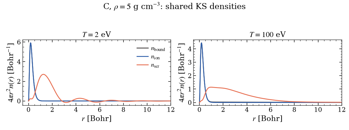
All LFC branches share the same electronic density at each temperature. The shell-weighted profiles make the radial electron numbers legible.
with style_context("thesis", palette="bing"):
    fig_density, density_axes = plt.subplots(
        1,
        len(states),
        figsize=grid_figsize(1, len(states)),
        squeeze=False,
    )
    for axis, state in zip(density_axes[0], states, strict=True):
        electronic_r = np.asarray(state["electronic_r_bohr"], dtype=float)
        shell_weight = 4.0 * np.pi * electronic_r**2
        mask = electronic_r <= 12.0
        for key, label in (
            ("n_bound_bohr3", r"$n_{\rm bound}$"),
            ("n_ion_bohr3", r"$n_{\rm ion}$"),
            ("n_scr_bohr3", r"$n_{\rm scr}$"),
        ):
            axis.plot(
                electronic_r[mask],
                (shell_weight * np.asarray(state[key], dtype=float))[mask],
                label=label,
            )
        axis.set(
            xlim=(-0.5, 12.0),
            xlabel=r"$r$ [Bohr]",
            ylabel=r"$4\pi r^2n(r)$ [Bohr$^{-1}$]",
            title=rf"$T={float(state['temperature_ev']):g}$ eV",
        )
    density_axes[0, 0].legend(frameon=False)
    fig_density.suptitle(
        rf"C, $\rho={RHO_G_CC:g}$ g cm$^{{-3}}$: shared KS densities",
        y=0.985,
    )
    fig_density.tight_layout(rect=(0.0, 0.0, 1.0, 0.94))
    save_figure(
        fig_density,
        FIGURE_DIR / "carbon_lfc_electronic_structure",
        close=False,
    )
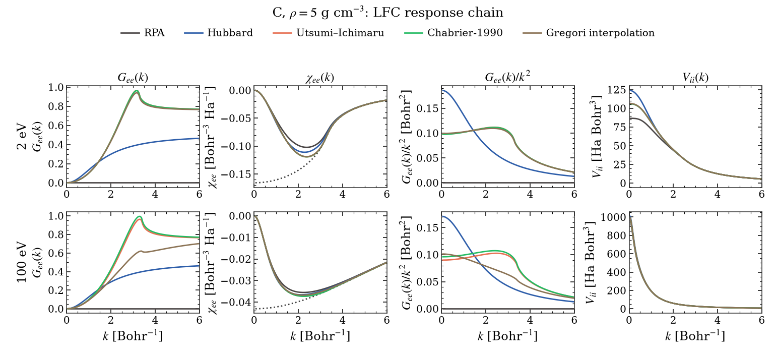
The response chain exposes the effect of each LFC on \(G_{ee}\), \(\chi_{ee}\), \(G_{ee}/k^2\), and \(V_{ii}\). The finite small-\(k\) limit of \(G_{ee}/k^2\) is the quantity that enters the LFC contribution to the effective potential.
with style_context("thesis", palette="bing"):
    colors = dict(
        zip(model_labels, plt.rcParams["axes.prop_cycle"].by_key()["color"])
    )
    fig_response, response_axes = plt.subplots(
        len(states),
        4,
        figsize=grid_figsize(len(states), 4),
        squeeze=False,
    )
    for row, state in enumerate(states):
        k = np.asarray(state["k_bohr_inv"], dtype=float)
        decomposition = low_k_decomposition(state)
        response_axes[row, 1].plot(
            k,
            np.asarray(state["chi0_k"], dtype=float),
            color="0.25",
            ls=":",
            label=r"shared $\chi^0_{ee}$",
        )
        for model_index, model in enumerate(model_labels):
            label = MODEL_LABELS[model]
            color = colors[model]
            response_axes[row, 0].plot(
                k,
                np.asarray(state["gee_k"], dtype=float)[model_index],
                color=color,
                label=label,
            )
            response_axes[row, 1].plot(
                k,
                np.asarray(state["chi_ee_k"], dtype=float)[model_index],
                color=color,
                label=label,
            )
            response_axes[row, 2].plot(
                k,
                decomposition["g_over_k2"][model_index],
                color=color,
                label=label,
            )
            response_axes[row, 3].plot(
                k,
                np.asarray(state["vii_k_ha_bohr3"], dtype=float)[model_index],
                color=color,
                label=label,
            )
        temperature = float(state["temperature_ev"])
        response_axes[row, 0].set_ylabel(
            rf"{temperature:g} eV" + "\n" + r"$G_{ee}(k)$"
        )
        response_axes[row, 1].set_ylabel(
            r"$\chi_{ee}$ [Bohr$^{-3}$ Ha$^{-1}$]"
        )
        response_axes[row, 2].set_ylabel(
            r"$G_{ee}(k)/k^2$ [Bohr$^2$]"
        )
        response_axes[row, 3].set_ylabel(
            r"$V_{ii}$ [Ha Bohr$^3$]"
        )
        for axis in response_axes[row]:
            axis.set_xlim(0.0, 6.0)
    for axis, title in zip(
        response_axes[0],
        (
            r"$G_{ee}(k)$",
            r"$\chi_{ee}(k)$",
            r"$G_{ee}(k)/k^2$",
            r"$V_{ii}(k)$",
        ),
        strict=True,
    ):
        axis.set_title(title)
    for axis in response_axes[-1]:
        axis.set_xlabel(r"$k$ [Bohr$^{-1}$]")
    handles, labels = response_axes[0, 0].get_legend_handles_labels()
    fig_response.legend(
        handles,
        labels,
        loc="upper center",
        bbox_to_anchor=(0.5, 0.945),
        ncol=5,
        frameon=False,
    )
    fig_response.suptitle(
        rf"C, $\rho={RHO_G_CC:g}$ g cm$^{{-3}}$: LFC response chain",
        y=0.985,
    )
    fig_response.tight_layout(rect=(0.0, 0.0, 1.0, 0.91))
    save_figure(
        fig_response,
        FIGURE_DIR / "carbon_lfc_response",
        close=False,
    )
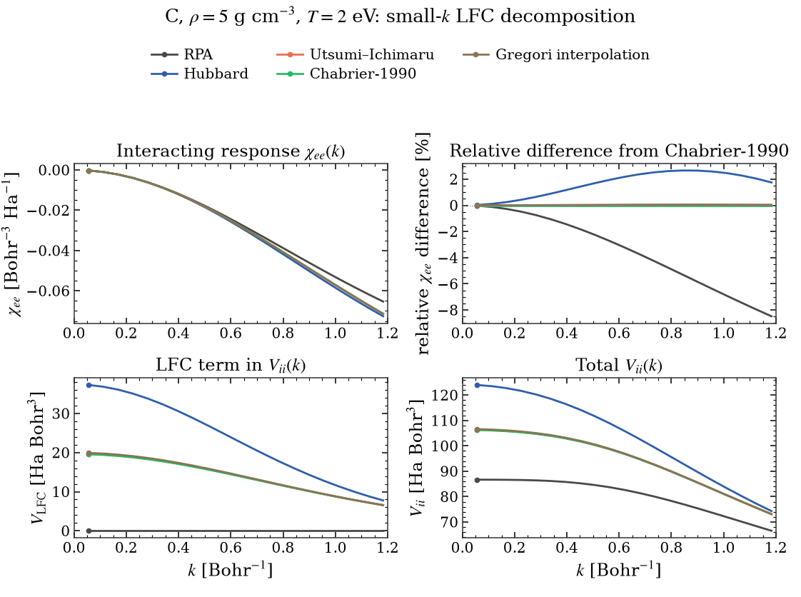
Why can nearly identical \(\chi_{ee}\) produce different \(V_{ii}\)?
The Starrett–Saumon reduction contains the inverse response,
Every Coulomb LFC considered here has \(G(k)=a k^2+O(k^4)\). Consequently all models share the leading \(\chi_{ee}(k)=-k^2/(4\pi)+O(k^4)\), so the response curves overlap. The LFC-dependent part of the potential nevertheless has the finite limit
The panels below show the cold-state response, the LFC contribution, and the resulting total potential. The remaining terms are identical for all branches because \(q(k)\), \(\bar Z\), and \(\chi_0(k)\) are held fixed.
with style_context("thesis", palette="bing"):
    colors = dict(
        zip(model_labels, plt.rcParams["axes.prop_cycle"].by_key()["color"])
    )
    fig_low_k, low_k_axes = plt.subplots(
        2,
        2,
        figsize=grid_figsize(2, 2),
        squeeze=False,
    )
    low_k_mask = cold_k <= LOW_K_PLOT_MAX_BOHR_INV
    shared_non_lfc = np.asarray(cold_low_k["shared_non_lfc"], dtype=float)
    if not np.allclose(
        shared_non_lfc,
        shared_non_lfc[reference_index],
        rtol=1.0e-12,
        atol=1.0e-10,
    ):
        raise RuntimeError("Expected a shared low-k charge/chi0 term.")
    for model_index, model in enumerate(model_labels):
        label = MODEL_LABELS[model]
        color = colors[model]
        plot_options = {
            "color": color,
            "label": label,
            "marker": "o",
            "markevery": [0],
            "ms": 4.0,
        }
        low_k_axes[0, 0].plot(
            cold_k[low_k_mask],
            cold_chi[model_index, low_k_mask],
            **plot_options,
        )
        low_k_axes[0, 1].plot(
            cold_k[low_k_mask],
            100.0
            * (
                cold_chi[model_index, low_k_mask]
                / cold_chi[reference_index, low_k_mask]
                - 1.0
            ),
            **plot_options,
        )
        low_k_axes[1, 0].plot(
            cold_k[low_k_mask],
            cold_low_k["lfc"][model_index, low_k_mask],
            **plot_options,
        )
        low_k_axes[1, 1].plot(
            cold_k[low_k_mask],
            cold_vii[model_index, low_k_mask],
            **plot_options,
        )
    low_k_axes[0, 0].set(
        ylabel=r"$\chi_{ee}$ [Bohr$^{-3}$ Ha$^{-1}$]",
        title=r"Interacting response $\chi_{ee}(k)$",
    )
    low_k_axes[0, 1].set(
        ylabel=r"relative $\chi_{ee}$ difference [%]",
        title="Relative difference from Chabrier-1990",
    )
    low_k_axes[1, 0].set(
        xlabel=r"$k$ [Bohr$^{-1}$]",
        ylabel=r"$V_{\rm LFC}$ [Ha Bohr$^3$]",
        title=r"LFC term in $V_{ii}(k)$",
    )
    low_k_axes[1, 1].set(
        xlabel=r"$k$ [Bohr$^{-1}$]",
        ylabel=r"$V_{ii}$ [Ha Bohr$^3$]",
        title=r"Total $V_{ii}(k)$",
    )
    for axis in low_k_axes.flat:
        axis.set_xlim(0.0, LOW_K_PLOT_MAX_BOHR_INV)
    low_k_axes[0, 1].axhline(0.0, color="0.55", lw=0.8, ls=":")
    handles, labels = low_k_axes[1, 1].get_legend_handles_labels()
    fig_low_k.legend(
        handles,
        labels,
        loc="upper center",
        bbox_to_anchor=(0.5, 0.94),
        ncol=3,
        frameon=False,
    )
    fig_low_k.suptitle(
        rf"C, $\rho={RHO_G_CC:g}$ g cm$^{{-3}}$, "
        rf"$T={float(cold_state['temperature_ev']):g}$ eV: "
        r"small-$k$ LFC decomposition",
        y=0.99,
    )
    fig_low_k.tight_layout(rect=(0.0, 0.0, 1.0, 0.85))
    save_figure(
        fig_low_k,
        FIGURE_DIR / "carbon_lfc_low_k_audit",
        close=False,
    )
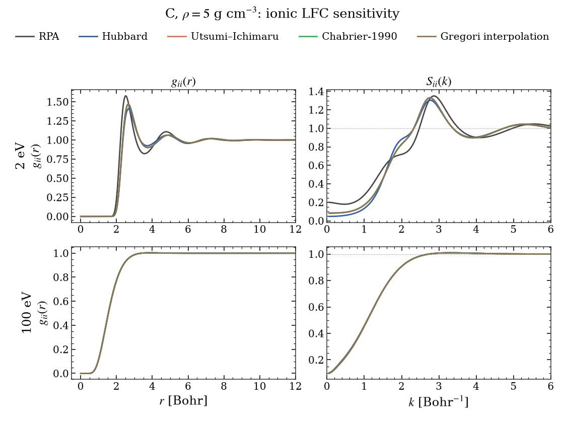
The same branches now feed HNC. Comparing 2 and 100 eV displays both a strongly LFC-sensitive regime and a regime in which the curves nearly coincide, without treating any approximation as exact reference data.
with style_context("thesis", palette="bing"):
    colors = dict(
        zip(model_labels, plt.rcParams["axes.prop_cycle"].by_key()["color"])
    )
    fig_ionic, ionic_axes = plt.subplots(
        len(states),
        2,
        figsize=grid_figsize(len(states), 2),
        squeeze=False,
    )
    for row, state in enumerate(states):
        r = np.asarray(state["r_bohr"], dtype=float)
        k = np.asarray(state["k_bohr_inv"], dtype=float)
        for model_index, model in enumerate(model_labels):
            label = MODEL_LABELS[model]
            color = colors[model]
            ionic_axes[row, 0].plot(
                r,
                np.asarray(state["gii_r"], dtype=float)[model_index],
                color=color,
                label=label,
            )
            ionic_axes[row, 1].plot(
                k,
                np.asarray(state["sii_k"], dtype=float)[model_index],
                color=color,
                label=label,
            )
        temperature = float(state["temperature_ev"])
        ionic_axes[row, 0].set_ylabel(
            rf"{temperature:g} eV" + "\n" + r"$g_{ii}(r)$"
        )
        ionic_axes[row, 0].set_xlim(-0.5, 12.0)
        ionic_axes[row, 1].set_xlim(0.0, 6.0)
        ionic_axes[row, 1].axhline(1.0, color="0.55", lw=0.8, ls=":")
    ionic_axes[0, 0].set_title(r"$g_{ii}(r)$")
    ionic_axes[0, 1].set_title(r"$S_{ii}(k)$")
    ionic_axes[-1, 0].set_xlabel(r"$r$ [Bohr]")
    ionic_axes[-1, 1].set_xlabel(r"$k$ [Bohr$^{-1}$]")
    handles, labels = ionic_axes[0, 0].get_legend_handles_labels()
    fig_ionic.legend(
        handles,
        labels,
        loc="upper center",
        bbox_to_anchor=(0.5, 0.945),
        ncol=5,
        frameon=False,
    )
    fig_ionic.suptitle(
        rf"C, $\rho={RHO_G_CC:g}$ g cm$^{{-3}}$: ionic LFC sensitivity",
        y=0.985,
    )
    fig_ionic.tight_layout(rect=(0.0, 0.0, 1.0, 0.91))
    save_figure(
        fig_ionic,
        FIGURE_DIR / "carbon_lfc_ionic_structure",
        close=False,
    )

if "agg" not in plt.get_backend().lower():
    plt.show()