Al: complete electronic-to-ionic workflow

This example follows one aluminium state through the complete Otter pipeline:

\[\mathrm{KS\!-\!DFT\ AA} \rightarrow \{n_{\rm ion},n_{\rm scr}\} \rightarrow V_{ii} \rightarrow \mathrm{OZ/HNC} \rightarrow \{g_{ii},S_{ii}\}.\]

The state is rho=8.1 g/cc and Te=Ti=1 eV. Set RECOMPUTE_WITH_OTTER=True below to run the calculation in this file. The default verifies and loads a reviewed result generated by the same workflow so documentation builds remain quick.

The full/external pseudoatom partition, continuum density, asymptotic density tail, and QOZ construction follow Starrett and Saumon [2014]. The default finite-temperature jellium local-field correction follows Chabrier [1990].

In addition to the two overview figures, the script writes slide-sized, single-purpose electronic-density, \(g_{ii}(r)\), and \(S_{ii}(k)\) figures as matching PNG/PDF pairs under the workflow output directory.

from __future__ import annotations

import hashlib
import json
import os
from pathlib import Path
import time
from typing import Any

import matplotlib.pyplot as plt
import numpy as np

from otter import PlasmaWorkflowConfig, solve_plasma_workflow
from otter.io.state import StateExportOptions, build_state_arrays
from otter.plotting import grid_figsize, save_figure, style_context


# =============================================================================
# User input
# =============================================================================
RECOMPUTE_WITH_OTTER = False
if os.environ.get("OTTER_RECOMPUTE_AL_FULL", "0") == "1":
    RECOMPUTE_WITH_OTTER = True

ELEMENT = "Al"
RHO_G_CC = 8.1
TE_EV = 1.0
TI_EV = 1.0

CONTINUUM_WORKERS = 4
HNC_TOL = 1.0e-6
HNC_CLOSURE_TOL = 1.0e-3
# =============================================================================


SCHEMA = "otter_al_full_workflow_v2"
HARTREE_TO_EV = 27.211386245988


def repository_root() -> Path:
    """Locate this Otter checkout when run directly or by Sphinx-Gallery."""
    candidates = [Path.cwd().resolve(), *Path.cwd().resolve().parents]
    source_file = globals().get("__file__")
    if source_file is not None:
        source = Path(str(source_file)).resolve()
        candidates.extend([source.parent, *source.parents])
    for candidate in candidates:
        if (
            candidate
            / "benchmarks"
            / "baselines"
            / "al_full_workflow_1ev"
            / "manifest.json"
        ).is_file():
            return candidate
    raise FileNotFoundError("Cannot locate the Otter repository root.")


ROOT = repository_root()
BASELINE_DIR = ROOT / "benchmarks" / "baselines" / "al_full_workflow_1ev"
OUTPUT_DIR = ROOT / "benchmarks" / "outputs" / "al_full_workflow_1ev"
FIGURE_DIR = OUTPUT_DIR / "figures"
RECOMPUTED_PATH = OUTPUT_DIR / "recomputed" / "Al_rho8p1gcc_Te1eV_Ti1eV.npz"


def sha256_file(path: Path) -> str:
    """Return a streaming SHA-256 checksum."""
    digest = hashlib.sha256()
    with path.open("rb") as stream:
        for block in iter(lambda: stream.read(1024 * 1024), b""):
            digest.update(block)
    return digest.hexdigest()


def load_reviewed_state() -> dict[str, np.ndarray]:
    """Verify and load the reviewed current-Otter result."""
    manifest = json.loads(
        (BASELINE_DIR / "manifest.json").read_text(encoding="utf-8")
    )
    record = manifest["state"]
    path = BASELINE_DIR / str(record["data_file"])
    if sha256_file(path) != str(record["data_sha256"]):
        raise RuntimeError(f"Checksum mismatch for {path}.")
    with np.load(path, allow_pickle=False) as archive:
        state = {key: np.asarray(archive[key]) for key in archive.files}
    if str(state["schema_version"].item()) != SCHEMA:
        raise ValueError("Unsupported Al full-workflow archive.")
    if any(value.dtype.hasobject for value in state.values()):
        raise TypeError("Object arrays are forbidden in gallery archives.")
    return state


def workflow_config() -> PlasmaWorkflowConfig:
    """Return the complete public Otter configuration used on this page."""
    return PlasmaWorkflowConfig(
        elements=[ELEMENT],
        temperature_ev=TE_EV,
        ion_temperature_ev=TI_EV,
        rho_g_cc=RHO_G_CC,
        aa_overrides={
            "cont_n_jobs": CONTINUUM_WORKERS,
            "cont_shards": 2 * CONTINUUM_WORKERS,
        },
        hnc_tol=HNC_TOL,
        hnc_closure_transform_tol=HNC_CLOSURE_TOL,
        hnc_max_iter=1000,
        show_progress=True,
    )


def finite_bound_levels(electronic: dict[str, Any]) -> dict[str, np.ndarray]:
    """Flatten finite negative-energy levels and ordinary FD occupations."""
    energies = np.asarray(electronic["bound_energy_ha"], dtype=float)
    l_values = np.asarray(electronic["bound_l_list"], dtype=int)
    fd = np.asarray(electronic["bound_fd"], dtype=float)
    occupation = np.asarray(electronic["bound_occ_deg_fd"], dtype=float)
    records: list[tuple[int, int, float, float, float]] = []
    for l_index, l_value in enumerate(l_values):
        for radial_index in range(energies.shape[1]):
            energy = float(energies[l_index, radial_index])
            if np.isfinite(energy) and energy < 0.0:
                records.append(
                    (
                        int(l_value),
                        int(radial_index + 1),
                        energy,
                        float(fd[l_index, radial_index]),
                        float(occupation[l_index, radial_index]),
                    )
                )
    values = np.asarray(records, dtype=float)
    return {
        "bound_l": values[:, 0].astype(int),
        "bound_n_index": values[:, 1].astype(int),
        "bound_energy_ha": values[:, 2],
        "bound_fd": values[:, 3],
        "bound_occ_deg_fd": values[:, 4],
    }


def pack_workflow(
    workflow: dict[str, Any],
    *,
    elapsed_s: float,
) -> dict[str, np.ndarray]:
    """Pack the plotted fields without relying on an external producer."""
    electronic = dict(workflow["electronic"]["result"])
    ion = dict(workflow["ion"])
    portable = build_state_arrays(
        workflow,
        options=StateExportOptions(r_max_bohr=20.0, k_max_bohr_inv=20.0),
    )
    r_e = np.asarray(electronic["r"], dtype=float)
    r = np.asarray(ion["r"], dtype=float)
    k = np.asarray(ion["k"], dtype=float)
    e_mask = r_e <= 20.0
    r_mask = r <= 20.0
    k_mask = k <= 20.0
    threshold_status = str(
        electronic.get("threshold_state_status", "none")
    ).strip().lower()
    charge_fix = dict(ion["charge_fix"])
    q_scale = float(charge_fix["scale_factor"])
    if not np.isfinite(q_scale) or q_scale <= 0.0:
        raise RuntimeError("The QOZ screening-charge scale is not physical.")
    q_used = np.asarray(ion["n_scr_k"], dtype=float)
    q_raw = q_used / q_scale
    if threshold_status == "unresolved":
        raise RuntimeError(
            "The final average atom has an unresolved threshold state."
        )
    if float(ion["hnc_best_residual"]) > HNC_TOL:
        raise RuntimeError("The final HNC residual exceeds the stated tolerance.")
    if float(ion["closure_transform_max_abs"]) > HNC_CLOSURE_TOL:
        raise RuntimeError(
            "The final finite-transform g(r)/S(k) mismatch exceeds tolerance."
        )

    def profile(name: str, fallback: str | None = None) -> np.ndarray:
        key = name if name in electronic else fallback
        if key is None or key not in electronic:
            raise KeyError(f"Electronic result has no {name!r} profile.")
        return np.asarray(electronic[key], dtype=float)[e_mask]

    payload: dict[str, np.ndarray] = {
        "schema_version": np.asarray(SCHEMA),
        "benchmark_id": np.asarray("al_full_workflow_1ev"),
        "state_id": np.asarray("al_full_workflow_rho8p1_te1_ti1"),
        "element": np.asarray(ELEMENT),
        "rho_g_cc": np.asarray(RHO_G_CC),
        "te_ev": np.asarray(TE_EV),
        "ti_ev": np.asarray(TI_EV),
        "producer_signature_json": np.asarray(
            json.dumps(
                {
                    "electronic_model": "qm",
                    "structure_model": "IS",
                    "aa_n_points": 4096,
                    "continuum_workers": CONTINUUM_WORKERS,
                    "bound_occ_mode": "fd",
                    "bound_rmax_mult": None,
                    "bound_zero_tail_refine": False,
                    "b3_tail_model": "full",
                    "qoz_n_points": 4096,
                    "chi0_model": "lindhard_fd",
                    "lfc_model": "chabrier1990",
                    "hnc_tol": HNC_TOL,
                    "hnc_closure_tol": HNC_CLOSURE_TOL,
                },
                sort_keys=True,
                separators=(",", ":"),
            )
        ),
        "producer_elapsed_s": np.asarray(elapsed_s),
        "r_e_bohr": r_e[e_mask],
        "n_full_bohr3": profile("n_full"),
        "n_free_bohr3": profile("n_cont"),
        "n_cont_bohr3": profile("n_cont"),
        "n_bound_bohr3": profile("n_bound"),
        "n_ext_bohr3": profile("n_ext"),
        "n_ion_bohr3": profile("n_ion"),
        "n_pa_bohr3": profile("n_pa"),
        "n_scr_bohr3": profile("n_scr"),
        "v_full_ha": profile("v_full", fallback="v_scf"),
        "v_ext_ha": profile("v_ext"),
        "v_hartree_ha": profile("v_H"),
        "v_xc_ha": profile("v_xc"),
        "n0_bohr3": np.asarray(float(electronic["n0"])),
        "r_ws_bohr": np.asarray(float(electronic["r_ws"])),
        "mu_ha": np.asarray(float(electronic["mu"])),
        "zbar_aa": np.asarray(float(electronic["zbar"])),
        "zbar_partition": np.asarray(float(ion["zbar_partition"])),
        "zbar_qoz": np.asarray(float(ion["zbar_qoz"])),
        "q_scr_raw": np.asarray(
            float(ion["zbar_screening_integral_raw"])
        ),
        "q_scr_grid_raw": np.asarray(float(charge_fix["q_scr_raw"])),
        "q_scr_used": np.asarray(float(charge_fix["q_scr_used"])),
        "q_scr_scale_factor": np.asarray(q_scale),
        "threshold_state_status": np.asarray(
            str(electronic.get("threshold_state_status", "none"))
        ),
        "threshold_state_representation": np.asarray(
            str(electronic.get("threshold_state_representation", "none"))
        ),
        "r_bohr": r[r_mask],
        "k_bohr_inv": k[k_mask],
        "gii_r": np.asarray(ion["gii_r"], dtype=float)[r_mask],
        "sii_k": np.asarray(ion["sii_k"], dtype=float)[k_mask],
        "vii_r_ha": np.asarray(ion["vii_r"], dtype=float)[r_mask],
        "vii_k_ha_bohr3": np.asarray(ion["vii_k"], dtype=float)[k_mask],
        "n_scr_k_electrons": q_used[k_mask],
        "n_scr_k_raw_electrons": q_raw[k_mask],
        "chi0_k_bohr3_per_ha": np.asarray(
            ion["chi0_k"], dtype=float
        )[k_mask],
        "gee_k": np.asarray(ion["gee_k"], dtype=float)[k_mask],
        "n_ion_k_electrons": np.asarray(
            portable["n_ion_k"], dtype=float
        )[0],
        "hnc_best_residual": np.asarray(float(ion["hnc_best_residual"])),
        "hnc_closure_mismatch": np.asarray(
            float(ion["closure_transform_max_abs"])
        ),
        "hnc_closure_tolerance": np.asarray(
            float(ion["closure_transform_tol"])
        ),
        "hnc_iters": np.asarray(int(ion["hnc_iters"])),
    }
    payload.update(finite_bound_levels(electronic))
    return payload


def calculate_state() -> dict[str, np.ndarray]:
    """Run AA -> pseudoatom -> QOZ/HNC and stage a portable result."""
    started = time.perf_counter()
    workflow = solve_plasma_workflow(workflow_config())
    state = pack_workflow(workflow, elapsed_s=time.perf_counter() - started)
    RECOMPUTED_PATH.parent.mkdir(parents=True, exist_ok=True)
    np.savez_compressed(RECOMPUTED_PATH, **state)
    print(f"Saved newly calculated state: {RECOMPUTED_PATH}")
    return state


state = calculate_state() if RECOMPUTE_WITH_OTTER else load_reviewed_state()
print(
    "Using "
    + (
        "a newly calculated Otter state."
        if RECOMPUTE_WITH_OTTER
        else "the checksummed current-Otter state."
    )
)


def level_rows() -> list[tuple[str, float, float, float, float]]:
    """Return spectroscopic labels and energies for terminal output."""
    symbols = ("s", "p", "d", "f", "g", "h")
    rows = []
    for l_value, radial_index, energy, fd, occupation in zip(
        state["bound_l"],
        state["bound_n_index"],
        state["bound_energy_ha"],
        state["bound_fd"],
        state["bound_occ_deg_fd"],
        strict=True,
    ):
        l_int = int(l_value)
        principal_n = int(radial_index) + l_int
        label = (
            f"{principal_n}{symbols[l_int]}"
            if l_int < len(symbols)
            else f"n={principal_n},l={l_int}"
        )
        rows.append(
            (
                label,
                float(energy),
                HARTREE_TO_EV * float(energy),
                float(fd),
                float(occupation),
            )
        )
    return rows


print(
    f"Al: rho={float(state['rho_g_cc']):g} g/cc, "
    f"Te=Ti={float(state['te_ev']):g} eV"
)
print(
    f"mu={float(state['mu_ha']):.8f} Ha, "
    f"HNC residual={float(state['hnc_best_residual']):.3e}"
)
print(
    "Zbar(AA-WS/partition/QOZ)="
    f"{float(state['zbar_aa']):.8f}/"
    f"{float(state['zbar_partition']):.8f}/"
    f"{float(state['zbar_qoz']):.8f}"
)
print(
    "Qscr(native/grid/used)="
    f"{float(state['q_scr_raw']):.8f}/"
    f"{float(state['q_scr_grid_raw']):.8f}/"
    f"{float(state['q_scr_used']):.8f}; "
    f"scale={float(state['q_scr_scale_factor']):.8f}"
)
print(
    f"{'level':>7s} {'E [Ha]':>13s} {'E [eV]':>13s} "
    f"{'FD':>10s} {'occupation':>12s}"
)
for row in level_rows():
    print(
        f"{row[0]:>7s} {row[1]:13.6f} {row[2]:13.6f} "
        f"{row[3]:10.6f} {row[4]:12.6f}"
    )

Using the checksummed current-Otter state.
Al: rho=8.1 g/cc, Te=Ti=1 eV
mu=1.04953778 Ha, HNC residual=8.058e-07
Zbar(AA-WS/partition/QOZ)=3.02607070/3.02284333/3.02284333
Qscr(native/grid/used)=3.02839880/3.02037354/3.02284333; scale=1.00081771
  level        E [Ha]        E [eV]         FD   occupation
     1s    -53.850704  -1465.352311   1.000000     2.000000
     2s     -2.734703    -74.415066   1.000000     2.000000
     2p     -1.363829    -37.111677   1.000000     6.000000

Electronic structure

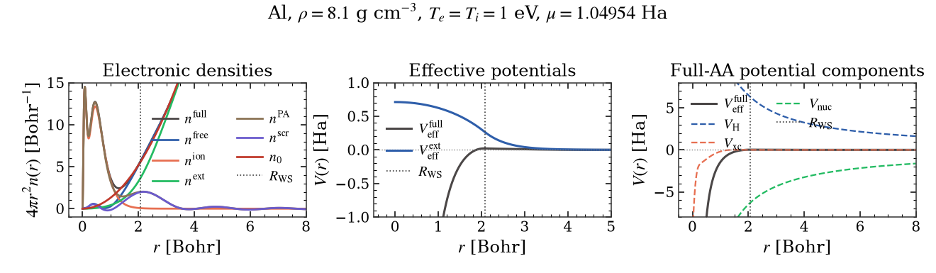
Solid curves are the full and external effective potentials. The middle panel keeps the requested linear [-1, 1] Ha screening-scale window. The right panel widens that same linear scale so the dashed nuclear and Hartree components remain visible. These are solver components on the adopted outer-potential gauge; the panel is not asserted to be an exact algebraic decomposition after every tail and gauge operation.

with style_context("thesis", palette="bing"):
    r_e = np.asarray(state["r_e_bohr"], dtype=float)
    shell = 4.0 * np.pi * r_e**2
    r_ws = float(state["r_ws_bohr"])
    mask_e = r_e <= 8.0

    fig_electronic, (
        ax_density,
        ax_potential,
        ax_decomposition,
    ) = plt.subplots(
        1,
        3,
        figsize=grid_figsize(1, 3),
    )
    density_curves = (
        ("n_full_bohr3", r"$n^{\rm full}$"),
        ("n_free_bohr3", r"$n^{\rm free}$"),
        ("n_bound_bohr3", r"$n^{\rm ion}$"),
        ("n_ext_bohr3", r"$n^{\rm ext}$"),
        ("n_pa_bohr3", r"$n^{\rm PA}$"),
        ("n_scr_bohr3", r"$n^{\rm scr}$"),
        ("n0_bohr3", r"$n_0$"),
    )
    for key, label in density_curves:
        ax_density.plot(
            r_e[mask_e],
            (shell * np.asarray(state[key], dtype=float))[mask_e],
            label=label,
        )
    ax_density.axvline(
        r_ws, color="0.25", ls=":", lw=1.1, label=r"$R_{\rm WS}$"
    )
    ax_density.set(
        xlabel=r"$r$ [Bohr]",
        ylabel=r"$4\pi r^2n(r)$ [Bohr$^{-1}$]",
        xlim=(-0.5, 8.0),
        ylim=(-1.0, 15.0),
        title="Electronic densities",
    )
    ax_density.legend(ncol=2)

    safe_r = np.maximum(r_e, np.finfo(float).tiny)
    effective_potentials = (
        ("v_full_ha", r"$V_{\rm eff}^{\rm full}$"),
        ("v_ext_ha", r"$V_{\rm eff}^{\rm ext}$"),
    )
    for key, label in effective_potentials:
        ax_potential.plot(
            r_e[mask_e],
            np.asarray(state[key], dtype=float)[mask_e],
            ls="-",
            lw=2.0,
            label=label,
        )
    ax_potential.axhline(0.0, color="0.5", ls=":", lw=0.9)
    ax_potential.axvline(
        r_ws, color="0.25", ls=":", lw=1.1, label=r"$R_{\rm WS}$"
    )
    ax_potential.set(
        xlabel=r"$r$ [Bohr]",
        ylabel=r"$V(r)$ [Ha]",
        xlim=(-0.5, 5.0),
        ylim=(-1.0, 1.0),
        title="Effective potentials",
    )
    ax_potential.legend()

    ax_decomposition.plot(
        r_e[mask_e],
        np.asarray(state["v_full_ha"], dtype=float)[mask_e],
        ls="-",
        lw=2.0,
        label=r"$V_{\rm eff}^{\rm full}$",
    )
    ax_decomposition.plot(
        r_e[mask_e],
        np.asarray(state["v_hartree_ha"], dtype=float)[mask_e],
        ls="--",
        lw=1.5,
        label=r"$V_{\rm H}$",
    )
    ax_decomposition.plot(
        r_e[mask_e],
        np.asarray(state["v_xc_ha"], dtype=float)[mask_e],
        ls="--",
        lw=1.5,
        label=r"$V_{\rm xc}$",
    )
    ax_decomposition.plot(
        r_e[mask_e],
        (-13.0 / safe_r)[mask_e],
        ls="--",
        lw=1.5,
        label=r"$V_{\rm nuc}$",
    )
    ax_decomposition.axhline(0.0, color="0.5", ls=":", lw=0.9)
    ax_decomposition.axvline(
        r_ws, color="0.25", ls=":", lw=1.1, label=r"$R_{\rm WS}$"
    )
    ax_decomposition.set(
        xlabel=r"$r$ [Bohr]",
        ylabel=r"$V(r)$ [Ha]",
        xlim=(-0.5, 8.0),
        ylim=(-8.0, 8.0),
        title="Full-AA potential components",
    )
    ax_decomposition.legend(ncol=2)

    fig_electronic.suptitle(
        rf"Al, $\rho={float(state['rho_g_cc']):g}$ g cm$^{{-3}}$, "
        rf"$T_e=T_i={float(state['te_ev']):g}$ eV, "
        rf"$\mu={float(state['mu_ha']):.5f}$ Ha",
        y=0.99,
    )
    fig_electronic.tight_layout(rect=(0.0, 0.0, 1.0, 0.965))
    save_figure(
        fig_electronic,
        FIGURE_DIR / "al_full_workflow_electronic",
        close=False,
    )

Pseudoatom to ion structure

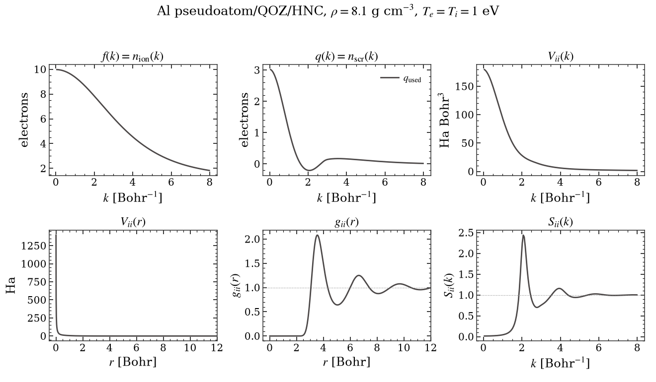
Here f(k)=n_ion(k) and q(k)=n_scr(k) use electron-number Fourier normalization. q_raw is the interpolated pseudoatom cloud before the documented scalar charge-closure correction; q_used is the cloud that enters QOZ and integrates to the selected pseudoatom-partition ionization. The interaction then enters the one-component OZ/HNC solve.

with style_context("thesis", palette="bing"):
    k = np.asarray(state["k_bohr_inv"], dtype=float)
    r = np.asarray(state["r_bohr"], dtype=float)
    k_mask = k <= 8.0
    r_mask = r <= 12.0
    fig_pipeline, axes = plt.subplots(
        2,
        3,
        figsize=grid_figsize(2, 3),
    )
    ax_f, ax_q, ax_vk, ax_vr, ax_g, ax_s = axes.ravel()

    ax_f.plot(k[k_mask], np.asarray(state["n_ion_k_electrons"])[k_mask])
    ax_f.set(
        title=r"$f(k)=n_{\rm ion}(k)$",
        xlabel=r"$k$ [Bohr$^{-1}$]",
        ylabel="electrons",
    )

    ax_q.plot(
        k[k_mask],
        np.asarray(state["n_scr_k_electrons"])[k_mask],
        label=r"$q_{\rm used}$",
    )
    ax_q.set(
        title=r"$q(k)=n_{\rm scr}(k)$",
        xlabel=r"$k$ [Bohr$^{-1}$]",
        ylabel="electrons",
    )
    ax_q.legend()

    ax_vk.plot(k[k_mask], np.asarray(state["vii_k_ha_bohr3"])[k_mask])
    ax_vk.set(
        title=r"$V_{ii}(k)$",
        xlabel=r"$k$ [Bohr$^{-1}$]",
        ylabel=r"Ha Bohr$^3$",
    )

    ax_vr.plot(r[r_mask], np.asarray(state["vii_r_ha"])[r_mask])
    ax_vr.set(
        title=r"$V_{ii}(r)$",
        xlabel=r"$r$ [Bohr]",
        ylabel="Ha",
        xlim=(-0.5, 12.0),
    )

    ax_g.plot(r[r_mask], np.asarray(state["gii_r"])[r_mask])
    ax_g.axhline(1.0, color="0.5", lw=0.8, ls=":")
    ax_g.set(
        title=r"$g_{ii}(r)$",
        xlabel=r"$r$ [Bohr]",
        ylabel=r"$g_{ii}(r)$",
        xlim=(-0.5, 12.0),
    )

    ax_s.plot(k[k_mask], np.asarray(state["sii_k"])[k_mask])
    ax_s.axhline(1.0, color="0.5", lw=0.8, ls=":")
    ax_s.set(
        title=r"$S_{ii}(k)$",
        xlabel=r"$k$ [Bohr$^{-1}$]",
        ylabel=r"$S_{ii}(k)$",
    )

    fig_pipeline.suptitle(
        rf"Al pseudoatom/QOZ/HNC, "
        rf"$\rho={float(state['rho_g_cc']):g}$ g cm$^{{-3}}$, "
        rf"$T_e=T_i={float(state['te_ev']):g}$ eV",
        y=0.99,
    )
    fig_pipeline.tight_layout(rect=(0.0, 0.0, 1.0, 0.965))
    save_figure(
        fig_pipeline,
        FIGURE_DIR / "al_full_workflow_ionic_pipeline",
        close=False,
    )


if "agg" not in plt.get_backend().lower():
    plt.show()